PAPER:
Some explicitly
solvable SABR and multiscale SABR models: option pricing and calibration
Lorella Fatone,
Francesca Mariani, Maria
Cristina Recchioni, Francesco
Zirilli
- Abstract
- Normal SABR model: new closed form formulae for
the transition probability density function and for the European option
prices
- Lognormal SABR model: new closed form formulae
for the transition probability density function and for the European
option prices
- Normal and lognormal multiscale SABR models: closed
form formulae for the transition probability density functions and for the
European option prices
- Calibration problem and forecasting
experiments using EUR/USD
currency's exchange rate and U.S.A. - five-Year
Interest Rate Swap data (movies)
- References
Warning: If your browser does not allow you
to see the content of this website click here to download a word file that
reproduces the material contained here.
A multiscale SABR model that describes the dynamics of forward
prices/rates is introduced. The model is a system of three stochastic
differential equations whose independent variable is time and whose dependent
variables are the forward prices/rates and two stochastic volatilities varying
on two different time scales. The two volatility equations are a two factor
volatility model. This multiscale model generalizes the SABR model introduced
in 2002 by Hagan, Kumar, Lesniewski, Woodward in [5]. The
SABR model is a system of two stochastic differential equations whose dependent
variables are the forward prices/rates and the stochastic volatility. The
volatility equation of the SABR model is a one factor volatility model.
Empirical studies have shown that in several circumstances two factors
volatility models describe the behaviour of financial prices more accurately
than one factor volatility models (see, for example, [1], [2], [3], [4], [8]). These studies motivate the introduction of the
multiscale SABR models. The SABR model [5] is
characterized by a correlation coefficient and by two parameters: the b volatility b Î [0,1] and the volatility of volatility e. The normal and lognormal
SABR models correspond respectively to the choices b = 0 and b = 1. The normal and lognormal
multiscale SABR models are the straightforward generalizations to the
multiscale context of the corresponding SABR models. We study the normal and
lognormal SABR and multiscale SABR models. Under some hypotheses on the
correlation coefficients of the Wiener processes appearing in the models,
``easy to use" closed form formulae for the transition probability density
functions of the state variables of the normal and lognormal multiscale SABR
models and for the prices of the corresponding European call and put options
are deduced. The formulae for the transition probability density functions are
three dimensional integrals of explicit integrands. Due to the special form of
the integrands these three dimensional integrals can be evaluated with a
standard quadrature rule at the computational cost of a two dimensional
integral. The method used to study the multiscale SABR models is applied to the
study of the normal and lognormal SABR models. For these models some new closed
form formulae for the transition probability density functions of their state
variables and for the prices of the European call and put options are deduced.
The transition probability density functions of the normal and lognormal SABR
models are expressed as one dimensional integrals of explicit integrands. In
the normal SABR model case the transition probability density function formula
presented in Section 2 can be used instead of formula (120) of [6].
This last formula is the one commonly used in mathematical finance and is based
on the Mc Kean formula [5], [6] for
the heat kernel of the Poincaré plane. In the lognormal SABR model case the
formula presented in Section 3 for the transition
probability density function is a special case of a new formula that gives the
transition probability density function of the Hull and White stochastic
volatility model [7] in presence of (possibly nonzero)
correlation between the stochastic differentials appearing on the right hand
side of the prices/rates and volatility equations. Moreover for the normal and
lognormal SABR models formulae to price European call and put options are
deduced. The formulae for the transition probability density functions presented
here are based on some recent results of Yakubovic [10]
on the heat kernel of the Lebedev Kontorovich Transform. A calibration problem for
the normal and lognormal SABR and multiscale SABR models is studied. This
calibration problem uses as data a set of option prices. The formulation of the
calibration problem is based on the option pricing formulae mentioned above and
on the least squares method. The procedure developed to solve the calibration
problem is tested on real data. The real data studied are time series of
exchange rates between currencies (euro/U.S. dollar, for short EUR/USD), of
European call and put option prices on the Eurodollar futures price, of
data of the U.S.A. five year interest rate swap futures prices and of
the corresponding option prices. Forecast option prices obtained with the
previous option pricing formulae are compared with prices actually observed.
This comparison establishes the quality of the forecast prices, of the
calibration procedure and of the models used. In particular it makes possible a
comparison between SABR and multiscale SABR models that shows when the use of
the multiscale SABR model is justified. This website contains some auxiliary
material including some animations that helps the understanding of the results presented in [4].
A more general reference to the work of the authors and of their coauthors in
mathematical finance is the website: http://www.econ.univpm.it/recchioni/finance.
Keywords. Multiscale
stochastic volatility models, option pricing, calibration problem, FX data,
interest rate swap data.
AMS (MOS) Subject
Classification. 62F10, 35R30, 91B70.
M.S.C.
classification. 34M50, 60H10, 91B28.
JEL classification: C53, G12, C61
2. Normal SABR model:
new closed form formulae for the transition probability density function and
for the European option prices
In this Section we give closed
form formulae for the transition probability density function and for the
European option prices of the normal SABR model. The option prices are expressed as expected
values of the discounted payoff when the dynamics of the underlying asset price
is given by the normal SABR model. The formulae presented are elementary and
can be used instead of the formulae deduced by Hagan, Kumar, Lesniewski,
Woodward in [5].
Let R and R+ be the
sets of real and of positive real numbers respectively and t be a real variable
that denotes time.
Let the forward prices/rates be described by the stochastic process xt, t ≥ 0, and the
stochastic volatility associated to the forward prices/rates be given by the
stochastic process vt, t>0. The SABR model introduced in 2002 by
Hagan, Kumar, Lesniewski, Woodward [5] is defined by the following equations:

where the
quantities ![]() and
and ![]() are real constants
satisfying the following conditions: bÎ[0,1], e > 0. The stochastic processes Wt, Qt ,
t>0, are standard Wiener processes such that W0= Q0=
0, dWt, dQt ,
t>0, are their stochastic differentials and we assume that <dWt
dQt >= rdt, t>0, where <· > denotes the expected value of · and rÎ(-1,1) is a
constant known as correlation
coefficient. Equations (1) and (2) are equipped with the initial conditions:
are real constants
satisfying the following conditions: bÎ[0,1], e > 0. The stochastic processes Wt, Qt ,
t>0, are standard Wiener processes such that W0= Q0=
0, dWt, dQt ,
t>0, are their stochastic differentials and we assume that <dWt
dQt >= rdt, t>0, where <· > denotes the expected value of · and rÎ(-1,1) is a
constant known as correlation
coefficient. Equations (1) and (2) are equipped with the initial conditions:

where ![]() ,
, ![]() are random variables assumed
to be concentrated in a point with probability one. We assume that
are random variables assumed
to be concentrated in a point with probability one. We assume that ![]() >0. This assumption implies that the process
>0. This assumption implies that the process ![]() , t>0, remains positive with probability one for t>0. Note
that
, t>0, remains positive with probability one for t>0. Note
that ![]() is not observable in
the financial market and must be interpreted as a parameter of the model. The
normal SABR model is the model obtained choosing b=0 in equations
(1). That is the normal SABR model is
defined by the following equations:
is not observable in
the financial market and must be interpreted as a parameter of the model. The
normal SABR model is the model obtained choosing b=0 in equations
(1). That is the normal SABR model is
defined by the following equations:

equipped with the
initial conditions (3), (4). Let ![]() be the transition
probability density function of the
normal SABR model (5), (6), (3), (4), that is let
be the transition
probability density function of the
normal SABR model (5), (6), (3), (4), that is let ![]() be the probability density
of having
be the probability density
of having ![]() ,
, ![]() when
when ![]() ,
, ![]() , t, t’³0, t-t’>0. Note that when t’=0 we must choose
x’=
, t, t’³0, t-t’>0. Note that when t’=0 we must choose
x’=![]() , v’=
, v’=![]() . In [4]
starting
from the backward Kolmogorov equation associated to the process defined by (5),
(6), using elementary analysis, the
following formula is deduced:
. In [4]
starting
from the backward Kolmogorov equation associated to the process defined by (5),
(6), using elementary analysis, the
following formula is deduced:

where i is the imaginary unit, the function
gN is given by:

sinh is the
hyperbolic sine and ![]() is the second type modified Bessel function of purely imaginary order.
is the second type modified Bessel function of purely imaginary order.
The function ![]() is known as the ``heat
kernel for the Kontorovich-Lebedev transform" (see [10] p. 748). The
function
is known as the ``heat
kernel for the Kontorovich-Lebedev transform" (see [10] p. 748). The
function ![]() given in (7) can be
rewritten in terms of elementary functions as follows:
given in (7) can be
rewritten in terms of elementary functions as follows:

where cosh is the
hyperbolic cosine. To deduce the option pricing formulae that follow from (9)
we give the expression of the marginal
distribution MN of the random variable xt, t>0, of having xt=x, t>0, given that xt’ =x’, vt’=v’, t, t’³0, t-t’>0, that
is:

where mN
is the following function:

and the function ![]() is given by:
is given by:

Let us consider in
the normal SABR model a European call option expiring at time t=T>0 and
having strike price K. The value CN of this option at time t=0, expressed as expected value of
the discounted payoff, when at time t=0 the underlying prices/rates value is ![]() and the
stochastic volatility is
and the
stochastic volatility is ![]() , is given by:
, is given by:

where (x)+
is the maximum between x and zero. Using
(11) we can rewrite (13) as follows:

where

Note that since we have <xt>= ![]() , t>0, the price at
time t=0 of a European put option
expiring at time t=T and having strike price K when
, t>0, the price at
time t=0 of a European put option
expiring at time t=T and having strike price K when ![]() and
and ![]() can be obtained via
the put-call parity relation, that is via the relation:
can be obtained via
the put-call parity relation, that is via the relation:
![]()
In formulae (13), (14), (16) we have assumed that the discount factor is
equal to one and this corresponds to choose the risk free interest rate equal
to zero. This assumption can be easily removed. Note that the expected values
contained in formulae (13), (14), (16) are computed with respect to the measure
whose density is given by (9), that is with respect to the physical measure.
This is correct when during the life time of the options the risk free interest
rate is deterministic. In fact in this
case the physical and the risk neutral measures coincide (see [9]).
3. Lognormal SABR model: new closed form formulae for the
transition probability density function and for the European option prices
In this Section we give closed form formulae for the transition
probability density function and for the European option prices of the
lognormal SABR model. The lognormal SABR
model is obtained from (1), (2) when b=1, that is it is given by:

where ![]() >0 is a real constant. As mentioned in Section 2 Wt,
Qt , t>0, are standard Wiener processes such that W0=
Q0= 0, dWt, dQt
, t>0, are their stochastic differentials and we assume that <dWt
dQt >= rdt, t>0, where rÎ(-1,1) is a
constant known as correlation
coefficient. Equations (17) and (18) are equipped with the initial conditions:
>0 is a real constant. As mentioned in Section 2 Wt,
Qt , t>0, are standard Wiener processes such that W0=
Q0= 0, dWt, dQt
, t>0, are their stochastic differentials and we assume that <dWt
dQt >= rdt, t>0, where rÎ(-1,1) is a
constant known as correlation
coefficient. Equations (17) and (18) are equipped with the initial conditions:

where ![]() ,
, ![]() are random variables concentrated in a point with probability one.
We assume that
are random variables concentrated in a point with probability one.
We assume that ![]() ,
, ![]() are positive, this
implies that the stochastic processes
are positive, this
implies that the stochastic processes ![]() ,
, ![]() , t>0, remain
positive with probability one for t>0.
, t>0, remain
positive with probability one for t>0.
The formulae
presented in this Section hold for rÎ(-1,1) and are
closed form formulae (see [4] for further
details). Note that up to now closed form formulae for the lognormal SABR model
known in the scientific literature are restricted to the case r=0, when r ¹0 the known
formulae are power series expansions.
We define the
variable ![]() , t>0. Using the new variable
, t>0. Using the new variable ![]() , t>0, the stochastic differential equations (17), (18)
are rewritten as follows:
, t>0, the stochastic differential equations (17), (18)
are rewritten as follows:

and the initial
conditions (19), (20) are rewritten as follows:

Let ![]() be the transition
probability density function of the lognormal
SABR model (21), (22), (23), (24), that is the probability density of having
be the transition
probability density function of the lognormal
SABR model (21), (22), (23), (24), that is the probability density of having ![]() ,
, ![]() when
when ![]() ,
, ![]() , t, t’³0, t-t’>0. Note that when t’=0 we must choose
, t, t’³0, t-t’>0. Note that when t’=0 we must choose![]() ,
, ![]() . Starting from the backward Kolmogorov equation associated
to the process defined by (21), (22), using elementary analysis, in [4] the following formula is deduced:
. Starting from the backward Kolmogorov equation associated
to the process defined by (21), (22), using elementary analysis, in [4] the following formula is deduced:

where the
function gL is given by:

and

The function gL
is defined through the ``heat kernel for the Kontorovich-Lebedev
transform" (see [10] p. 748).
The function pL
can be rewritten in terms of elementary functions as follows:

To deduce the
option price formulae that follow from (28) we give the expression of the
marginal distribution ML of the random
variable xt, t>0, of having
xt=x given that xt’=x’, vt’=v’, t, t’³0, t-t’>0, that is:

where mL
is the following function:

and the function ![]() is given by:
is given by:

Let us consider in
the lognormal SABR model a European call option expiring at time t=T>0 and
having strike price K>0. The value CL
of this option at time t=0 when at time t=0 the underlying prices/rates value
is ![]() and the stochastic volatility is
and the stochastic volatility is ![]() is given by:
is given by:

Similarly in the
lognormal SABR model let PL denote the value at time t=0 of the
European put option expiring at time t=T>0 and having strike price K>0
when at time t=0 the underlying prices/rates value is ![]() and the stochastic
volatility is
and the stochastic
volatility is ![]() , its value is given by:
, its value is given by:

Note that as done
in Section
4. Normal and lognormal multiscale SABR models: closed form formulae for the
transition probability density function and for the European option prices
Let us
introduce the multiscale SABR model. We
associate to the forward prices/rates variable xt, t ≥ 0, two
stochastic volatilities v1,t, v2,t, t ≥ 0, one
fluctuating on a fast time scale and the other one fluctuating on a long time
scale. The dynamics of the stochastic process xt, v1,t, v2,t,
t > 0, is defined by the following system of stochastic differential
equations:

where the
quantities ![]() and
and ![]() , i = 1,2, are real constants such that: bÎ[0,1], ei > 0, i=1,2, e1 £ e2 .
, i = 1,2, are real constants such that: bÎ[0,1], ei > 0, i=1,2, e1 £ e2 .
Moreover Wt0,1,
Wt0,2 ,Wt1, Wt2,
t>0, are standard Wiener processes such that W00,1= W00,2=W01=W02=0, dWt0,1, dWt0,2
,dWt1, dWt2, t>0, are
their stochastic differentials and we assume that <dWt0,1dWt0,2
>= 0, <dWt0,1dWt1
>= r0,1dt, <dWt0,2dWt2
>= r0,2dt, <dWt1dWt2>=0 , t>0, r0,1, r0,2Î(-1,1) are constants
known as correlation coefficients.
The fact that the model is a two scale stochastic volatility model is
translated in the assumption that ![]() . The equations (34), (35), (36) must be equipped with the initial conditions:
. The equations (34), (35), (36) must be equipped with the initial conditions:

The random
variables ![]() ,
, ![]() ,
, ![]() are assumed to be
concentrated in a point with probability one.
We assume that
are assumed to be
concentrated in a point with probability one.
We assume that ![]() ,
, ![]() >0. The assumption
>0. The assumption ![]() ,
, ![]() >0 with probability
one implies that
>0 with probability
one implies that ![]() , v2,t are
positive with probability one for t > 0. Note that the quantities
, v2,t are
positive with probability one for t > 0. Note that the quantities ![]() ,
, ![]() are not observable in
the financial market and that they must be regarded as parameters of the model.
are not observable in
the financial market and that they must be regarded as parameters of the model.
The multiscale SABR model (34),
(35), (36)
generalizes the SABR model (1), (2).
We consider the normal and the
lognormal multiscale SABR models. These models are obtained from (34), (35),
(36) choosing in (34) respectively b = 0 and b = 1. When we consider the lognormal model we assume ![]() > 0. In the lognormal model the assumption
> 0. In the lognormal model the assumption ![]() > 0 with probability one (together with the
assumptions
> 0 with probability one (together with the
assumptions ![]() ,
, ![]() >0) implies that xt > 0 with probability one for t > 0. Under the previous
assumptions on the correlation structure for the normal and lognormal
multiscale SABR models the transition probability density functions of the
state variables of these models can be expressed via closed form integral
formulae with explicit integrands. In this sense the normal and lognormal
models are explicitly solvable.
>0) implies that xt > 0 with probability one for t > 0. Under the previous
assumptions on the correlation structure for the normal and lognormal
multiscale SABR models the transition probability density functions of the
state variables of these models can be expressed via closed form integral
formulae with explicit integrands. In this sense the normal and lognormal
models are explicitly solvable.
Let us consider the normal multiscale SABR model, we have:

with the initial conditions
(37), (38), (39).
Let ![]() be the transition
probability density function of the
normal multiscale SABR model (40), (41),
(42), (37), (38), (39), that is the probability density of having
be the transition
probability density function of the
normal multiscale SABR model (40), (41),
(42), (37), (38), (39), that is the probability density of having ![]() ,
, ![]() ,
, ![]() when
when ![]() ,
, ![]() ,
, ![]() , t, t’³0, t-t’>0. Note that
when t’=0 we must choose
, t, t’³0, t-t’>0. Note that
when t’=0 we must choose ![]() ,
, ![]() ,
, ![]() , Starting from the backward Kolmogorov equation associated
to the process defined by (40), (41), (42) , using elementary analysis, in [4] the following formula is deduced:
, Starting from the backward Kolmogorov equation associated
to the process defined by (40), (41), (42) , using elementary analysis, in [4] the following formula is deduced:

where the
function gN is given in (7).
Note that the
transition probability density function of the normal multiscale SABR model
given in (43) is expressed as the Fourier transform of the product of two
copies of the function gN evaluated in two different points. The two
copies of the function gN are coupled through the integration in the
variable k. The variable k is the
conjugate variable of the variable x’-x.
To deduce the option
price formulae that follow from (43) we give the expression of the marginal
distribution MMN in the normal multiscale SABR model of the variable
xt, t>0, of having xt =x given that ![]() ,
, ![]() ,
, ![]() , t, t’³0, t-t’>0, that is:
, t, t’³0, t-t’>0, that is:

where mN
is the function given in (11).
Let us consider in
the normal multiscale SABR model a European call option expiring at time t=T>0
and having strike price K. The value CMN
of this option at time t=0 when at time
t=0 the underlying prices/rates value is
![]() and the stochastic volatilities are
and the stochastic volatilities are ![]() ,
, ![]() is given by:
is given by:

Let PMN
denote the price in the normal multiscale SABR model at time t=0 of the
European put option expiring at time t=T>0 and having strike price K when at
time t=0 the underlying prices/rates value is ![]() and the stochastic
volatilities are
and the stochastic
volatilities are ![]() ,
, ![]() , we have:
, we have:

Note that, as
already done in Section 2 and 3,
in formulae (45), (46) we have assumed the discount factor equal to one and, as
a consequence, the risk free interest rate equal to zero. Moreover we have
assumed that the risk free interest rate is deterministic during the lifetime
of the options considered.
We conclude this Section
studying the lognormal multiscale SABR model, that is model (34), (35), (36) with b=1. We have:

with the initial conditions
(37), (38), (39). When we consider the lognormal multiscale SABR model we
assume ![]() >0. The assumption
>0. The assumption ![]() >0 with probability one (together with the assumption
>0 with probability one (together with the assumption ![]() ,
, ![]() >0) implies that
>0) implies that ![]() is positive with
probability one for t>0. Using the variable
is positive with
probability one for t>0. Using the variable ![]() , t>0, we can rewrite
the stochastic differential equation (47) as done in (21).
, t>0, we can rewrite
the stochastic differential equation (47) as done in (21).
Let ![]() be the transition
probability density function of the lognormal
multiscale SABR model (47), (48), (49), (37), (38), (39) expressed in the
variable
be the transition
probability density function of the lognormal
multiscale SABR model (47), (48), (49), (37), (38), (39) expressed in the
variable![]() , t>0, that is the probability density of having
, t>0, that is the probability density of having ![]() ,
, ![]() ,
, ![]() when
when ![]() ,
, ![]() ,
, ![]() , t, t’³0, t-t’>0. Note that when t’=0 we must choose
, t, t’³0, t-t’>0. Note that when t’=0 we must choose ![]() ,
, ![]() ,
, ![]() . Using elementary analysis applied to the backward
Kolmogorov equations associated to the process (47), (48), (49) expressed in
the variable
. Using elementary analysis applied to the backward
Kolmogorov equations associated to the process (47), (48), (49) expressed in
the variable ![]() , t>0, we deduce the following formula (see [4] for further
details):
, t>0, we deduce the following formula (see [4] for further
details):

where the
function gL is defined in (26).
To deduce the
option price formulae that follow from (50) we give the marginal distribution MML
of the variables xt=x, given that ![]() ,
, ![]() ,
, ![]() , t, t’³0, t-t’>0, that is:
, t, t’³0, t-t’>0, that is:

where mL
is the function given in (30).
Let us consider in
the lognormal multiscale SABR model a European call option expiring at time t=T>0
and having strike price K>0. The
value CML of this option at
time t=0 when at time t=0 the underlying prices/rates value is ![]() (recall x0=ln(x0 / x0)=0) and
the stochastic volatilities are
(recall x0=ln(x0 / x0)=0) and
the stochastic volatilities are ![]() ,
, ![]() is given by:
is given by:

where mL is
the function given in (30).
Let PML
denote the price in the lognormal multiscale SABR model at time t=0 of the
European put option expiring at time t=T>0 and having strike price K>0 when at time t=0 the underlying prices/rates
value is ![]() and the stochastic
volatilities are
and the stochastic
volatilities are ![]() ,
, ![]() , we have:
, we have:

Note that as done
in Section 2 and 3 in
formulae (52), (53) we have assumed the discount factor equal to one and, as a
consequence, the risk free interest rate equal to zero. Moreover we have
assumed that the risk free interest rate is deterministic during the lifetime
of the options considered.
The evaluation of
the option pricing formulae of Section 2, 3, 4, that is of the formulae (13),
(32), (33), (45), (46), (52), (53), can take advantage from several special features
of these formulae. In particular formulae (13), (32), (33), (45), (46), (52),
(53) are Fourier integrals that can be computed using the FFT algorithm.
Moreover the computational cost of evaluating these formulae for several
choices of the strike price K and of the spot price ![]() can be reduced noting
that the functions mN and mL given respectively in (11) and (30) that
appear in formulae (13), (32), (33),
(45), (46), (52), (53) are
independent of the strike price K and of the spot price
can be reduced noting
that the functions mN and mL given respectively in (11) and (30) that
appear in formulae (13), (32), (33),
(45), (46), (52), (53) are
independent of the strike price K and of the spot price ![]() so that they can be computed once and forever on a
grid of the k variable and then used to evaluate the option prices for several values
of the strike price K and of the spot prices
so that they can be computed once and forever on a
grid of the k variable and then used to evaluate the option prices for several values
of the strike price K and of the spot prices ![]() . Recall that formula (14) to price European call options in
the normal SABR model can be used instead of formula (13) and that formulae
analogous to (14) can be deduced for the remaining option price formulae
derived in Section 2, 3, 4.
. Recall that formula (14) to price European call options in
the normal SABR model can be used instead of formula (13) and that formulae
analogous to (14) can be deduced for the remaining option price formulae
derived in Section 2, 3, 4.
5. Calibration problem and forecasting experiments using EUR/USD currency's exchange rate and U.S.A. - five-Year Interest Rate Swap data (movies)
The calibration problems
considered in this Section use as data a set of option prices observed at a
given time. The option price data are fitted in the least squares sense with
the option pricing formulae presented in Section 2, 3 and 4 imposing the constraints on the model
parameters that are dictated from their “physical” meaning. In this Section the
risk free interest rate r is not assumed to be zero. In the case of the normal
and lognormal SABR models the constraints define the set M* of the feasible points as follows:
![]()
and in the case of the normal
and lognormal multiscale SABR model the
constraints define the set M** of the feasible points as follows:
![]()
where R4 and R7
are respectively the four and seven
dimensional real Euclidean space. The calibration problem is formulated as a
nonlinear constrained least squares problem whose feasible set is M* or M**. The independent variable of this least squares problem is ![]() (SABR models) or
(SABR models) or ![]() (multiscale SABR models).
(multiscale SABR models).
Note that the vector ![]() contains the model
parameters and the risk free interest rate and that, for simplicity, we use the
same symbol
contains the model
parameters and the risk free interest rate and that, for simplicity, we use the
same symbol ![]() to denote a vector
belonging to M* or to M**. The risk free interest rate appears
in the discount factor that multiplies the option pricing formulae given in the
previous Sections.
to denote a vector
belonging to M* or to M**. The risk free interest rate appears
in the discount factor that multiplies the option pricing formulae given in the
previous Sections.
When we calibrate the model
parameters of the normal SABR model the objective function is defined as the
square of the differences between the observed European call and put option
prices and the corresponding call and put option prices computed with formulae
(14), (16) completed with the appropriate discount factor. The same procedure
is used to calibrate all the remaining models presented in Section 3 and 4.
That is formulae (32), (33) are used to calibrate the log-normal SABR model and
formulae (45), (46) and (52), (53) are used to calibrate respectively the
normal and lognormal multiscale SABR models. Formulae (32), (33), (45), (46),
(52), (53) are completed with the appropriate discount factor depending on the
risk free interest rate that has been omitted in the previous Sections.
5.2 Numerical Results on future prices on the EUR/USD exchange
rate
In this experiment we consider the daily values of
the futures price on the EUR/USD currency's exchange rate having maturity
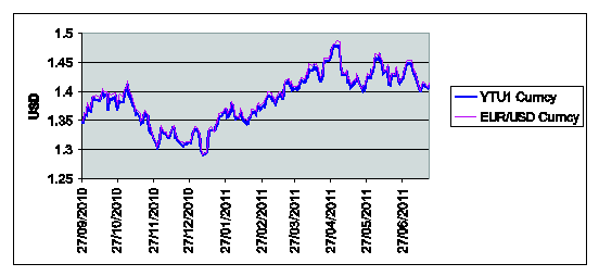
September 16th, 2011, (the third Friday of September 2011) (ticker YTU1 Curncy
of Figure 1) and the daily prices of the corresponding
European call and put options with expiry date September 9th, 2011 and strike
prices KC,i = KP,i = Ki = 1.375+0.005*(i-1), i
= 1,2,¼,18. The strike prices Ki, i = 1,2,¼, 18, are expressed in USD. These prices are observed in the time period
that goes from September 27th, 2010, to July 19th, 2011. The observations are
made daily and the prices considered are the closing prices of the day. Recall
that a year is made of about 250-260 trading days and a month is made of about
20-22 trading days. Figure1 shows the futures price
(ticker YTU1 Curncy) (blue line) and the EUR/USD currency's exchange rate (pink
line) as a function of time. Figures 2 and 3 show respectively the prices (in USD) of the
corresponding call and put options with maturity time September 9th, 2011 and
strike price Ki, i = 1,2,¼,18, as a function of time.
Figure 1: YTU1 (blue line) and EUR/USD currency's exchange rate (pink
line) versus time.
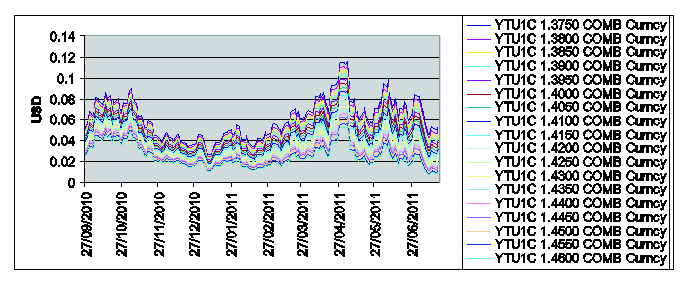
Figure 2: Call option prices on YTU1 with
strike price Ki = 1.375+0.005*(i-1), i = 1,2,¼,18, and expiry date T= September 9th, 2011 versus time.
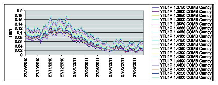
Figure 3: Put option prices
on YTU1 with strike price Ki = 1.375+0.005*(i-1), i = 1,2,¼,18, and expiry date T= September 9th, 2011 versus time.
We use the normal SABR and multiscale SABR models to study these data.
In
particular for these models we solve the calibration problem posed in Section 5.1 for t= tj, j = 1,2,3, where t1
= September 27th, 2010, t2 = October 25th, 2010, t3
= November 4th, 2010 using as data the EUR/USD futures prices (YTU1 ticker
of Figure 1) and the prices of the previously mentioned
eighteen call and eighteen put options (Figure 2 and Figure 3) available at t = tj, j = 1,2,3. The
choice of the dates t= tj, j = 1,2,3, exploits the fact that the option
pricing formulae deduced in Section 2, 3 and 4 are closed form formulae. That is these formulae do not
involve asymptotic expansions and can be used always. In particular they can be
used when the products e2 (T-t), ei2 (T-t), i = 1,2, where t is the current time and T is the
expiry date of the options are not small and this is the case when we consider
the choices made previously.
Table 1
and Table 2 show
respectively the parameter values obtained as solution of the calibration
problems considered above for the normal SABR and multiscale SABR models.
|
T* - date of calibration |
e |
|
r |
R |
|
September 27th, 2010 |
0.514 |
0.161 |
-0.415 |
0.0 |
|
October 25th, 2010 |
0.844 |
0.186 |
-0.355 |
0.033 |
|
November 4th, 2010 |
0.844 |
0.181 |
-0.267 |
0.019 |
Table 1:
Solution of the calibration problem: normal SABR model
|
t*- date of calibration |
e1 |
|
r0,1 |
R |
e2 |
|
r0,2 |
|
September 27th, 2010 |
0.514 |
0.143 |
-0.0164 |
0.0069 |
0.8842 |
0.083 |
-0.558 |
|
October 25th, 2010 |
0.513 |
0.164 |
-0.046 |
0.0077 |
0.892 |
0.087 |
-0.550 |
|
November 4th, 2010 |
0.507 |
0.158 |
-0.084 |
0.0112 |
0.894 |
0.087 |
-0.561 |
Table 2:
Solution of the calibration problem: normal multiscale SABR model
The calibrated models, that is
those with the parameter values given in Table 1
and Table 2, are used to forecast option prices one
day, two days,..., up to twenty one days ahead of the observation day of the
prices that are used to calibrate the model. Recall that we are considering
trading days and that twenty one trading days are approximately one month. The
forecasts are made evaluating formulae (45) and (46) when we consider the normal
multiscale SABR model and evaluating formulae (14) and (16) when we consider
the normal SABR model multiplied by the appropriate discount factor. Note that
in the forecasting experiment these formulae are evaluated using as underlying
asset value the futures price observed the day of the forecast. The
volatilities ![]() and
and ![]() obtained from the calibration
problem are taken as proxies of the volatilities the day of the forecast.
obtained from the calibration
problem are taken as proxies of the volatilities the day of the forecast.
In detail we forecast the option prices day by
day up to twenty one (trading) days ahead of t*=tj, j=1,2,3, (i.e. we consider t*+ Dt, t*+2Dt,...,t*+21Dt , where Dt = one day) using in the option pricing formulae evaluated at the futures price
observed the day of the forecast.
MOVIE 1 is made of twenty one frames and shows the futures prices Figure 1
(window on the upper-left corner), the observed and forecast prices of the
eighteen call
options considered in Figure 2 (window on the upper-right
corner) one day, two days,…, twenty one days ahead of the day of calibration
and the corresponding relative errors obtained using the normal SABR (window on
the lower-left corner) and normal multiscale SABR (window on the lower-right corner) models.
Click here to see MOVIE 1
MOVIE 2 is made of twenty one frames and shows the futures prices Figure 1 (window
on the upper-left corner), the observed and
forecast prices of the eighteen put
options considered in Figure 3 (window on the
upper-right corner) one day, two days,…,
twenty one days ahead of the day of calibration and the corresponding relative
errors obtained using the normal SABR (window on the lower-left corner) and
normal multiscale SABR (window on the
lower-right corner) models..
Click here to see MOVIE 2
Note that the mean relative
errors in the twenty one day forecasts obtained using the normal multiscale
SABR model show that this model guarantees about two significant digits correct
in the option prices. This is true also when the options are at the money, that
is when the moneyness is close to one. The fact that the normal multiscale
model outperforms the normal SABR model is evident when t* = t2, but
it is true also when t* = t1 or
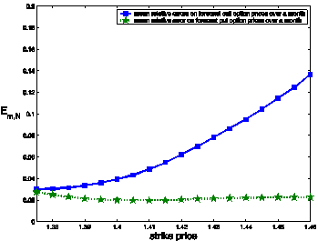
t* = t3. Figure 4 shows the mean relative
errors obtained with the calibration done at t*=t2. Note that when t*=t2
the futures price of the EUR/USD
exchange rate is 1.3901 and the options with strike price Ki = 1.375+0.005*(i-1), i
= 1,2,¼,6, can be
considered at the money.
 (a)
(a)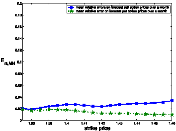 (b)
(b)
Figure 4: Mean
relative error on the forecast option prices over a period of one month (21
trading days). The forecasts are obtained using the model parameters resulting from the
calibration at t* = t2 = October 25th 2010 with normal
SABR model (a) and normal multiscale SABR model (b) versus strike price (FX
experiment).
When t =![]() , i=1,2,3, the values e1 and e2 of the two
volatilities of volatilities resulting from the calibration of the normal
multiscale SABR model differ substantially (i.e. the ratio e2/ e1 is greater than 1.6-1.7, see Table 1 and Table 2) and
the quality of the forecast option prices obtained using the normal
multiscale SABR model is higher than the quality of the forecast option prices
obtained using the normal SABR model. We have observed that when the multiscale
SABR model improves significantly the quality of the forecast option prices
obtained with the SABR model the value of the ratio e2/ e1 of the parameter values resulting from the
calibration is greater 1.6-1.7 (see [4] for further details). In fact in [4] we have repeated this experiment using the same data and the
lognormal SABR and multiscale SABR models instead of the normal SABR and
multiscale SABR models. We observe that the lognormal SABR model provides
forecast option prices of high quality and that the use of the multiscale SABR
model does not improve substantially the quality of the forecasts. In the
experiment with the lognormal models the ratio e2/ e1 resulting from the
calibration is approximately one.
, i=1,2,3, the values e1 and e2 of the two
volatilities of volatilities resulting from the calibration of the normal
multiscale SABR model differ substantially (i.e. the ratio e2/ e1 is greater than 1.6-1.7, see Table 1 and Table 2) and
the quality of the forecast option prices obtained using the normal
multiscale SABR model is higher than the quality of the forecast option prices
obtained using the normal SABR model. We have observed that when the multiscale
SABR model improves significantly the quality of the forecast option prices
obtained with the SABR model the value of the ratio e2/ e1 of the parameter values resulting from the
calibration is greater 1.6-1.7 (see [4] for further details). In fact in [4] we have repeated this experiment using the same data and the
lognormal SABR and multiscale SABR models instead of the normal SABR and
multiscale SABR models. We observe that the lognormal SABR model provides
forecast option prices of high quality and that the use of the multiscale SABR
model does not improve substantially the quality of the forecasts. In the
experiment with the lognormal models the ratio e2/ e1 resulting from the
calibration is approximately one.
5.3
Numerical Results on the
In this experiment we consider
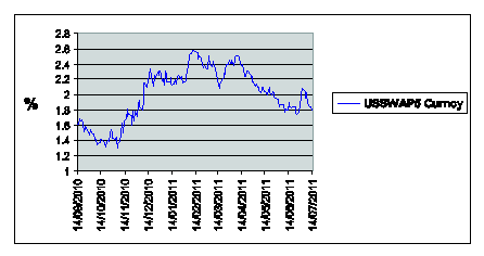
the daily observed values of the U.S.A. five-Year Interest Rate Swap expressed
in per cent (the ticker USSWAP5 curncy in Figure 5(a)),
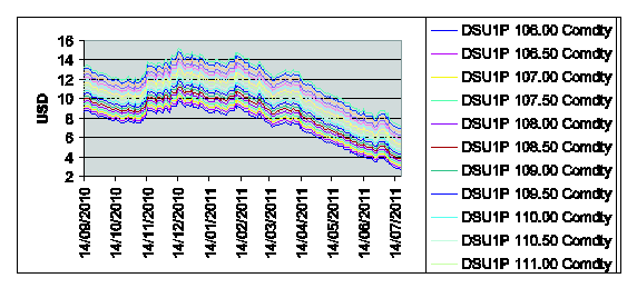
the corresponding futures prices having maturity September 30th, 2011 (the
ticker DSU1 in Figure 5(b)) and the prices of the
corresponding European call and put options with expiry date September 19th,
2011 and strike prices Ki = 106+0.5*(i-1), i = 1,2,¼,18. These prices are observed
in the period going from September 14th, 2010, to July 20th, 2011. The strike prices Ki, i = 1,2,¼, 18, are expressed in
hundreds of base points. For example, Ki = 106 corresponds to an
interest rate of 106-100 = 6 hundreds of base points, that is corresponds to an
interest rate of 6% per year (see Figure 5).
Note that from November 12th, 2010
to December 15th, 2010 the futures price goes from the value of 110 to the
value of 104 hundreds of base points.
 (a)
(a)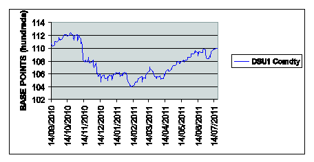 (b)
(b)
Figure 5: Observed
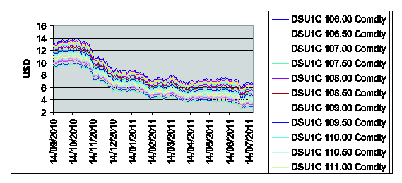
Figure 6: Call option prices on DSU1 with
strike price Ki = 106+0.5*(i-1), i = 1,2,¼,18, and expiry date T= September 19th, 2011 versus time.
Figure 7: Put option prices on DSU1 with strike
price Ki = 106+0.5*(i-1), i = 1,2,¼,18, and expiry date T= September 19th, 2011 versus time.
We use the
lognormal SABR and multiscale SABR models to study the data shown in Figure 5, 6, 7 [4].
This study shows that the lognormal
multiscale SABR model improves
substantially the quality of the forecast option prices obtained using the
lognormal SABR model and we observe that in this case the ratio e2/ e1 resulting from the calibration is greater than
1.6. That is the experiment on the
We present now an experiment that tackles the question of how the
results of the calibration reflect the model dynamics.
The experiment consists in calibrating the lognormal models every day
for approximately two months, that is we
calibrate the lognormal models in the
period going from September 14th, 2010 to November 15th, 2010 using the daily
data of the interest rate swap futures prices considered in this Subsection.
Note that in this period we can observe significant oscillations in the
value of the futures prices. In fact, for example, on October 12th, 2010 the futures price (ticker DSU1 Figure 5(b)) is 112.093 and on November 15th, 2010 the futures price is down to
107.875.
Note that in the first part of the period (September 14th,
2010- October 14th, 2010) the
oscillations of the futures price are small
and in the second part (October
14th, 2010- November 15th, 2010) in particular around the
end of October 2010 there is a fall of
the futures price (see Figure 5).
The parameter
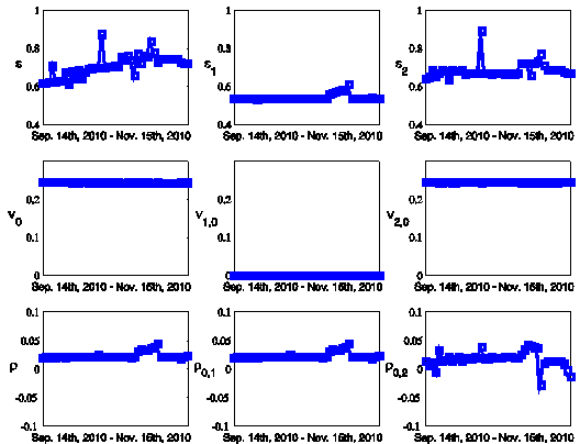
values obtained from the calibration of the lognormal models are shown in Figure 8. We can see that the values of the
parameters remain
substantially unchanged in the two months period except for the values of the
parameters e and e2 that show a
significant
change at the end of October 2010 and during
the first fifteen days of November 2010. Moreover we use the parameter values
obtained with the calibration of the lognormal SABR and multiscale SABR models to compute the forecast
option prices one day in the future during the two months period mentioned
above. Movie 3 and Movie 4 show
the forecast option prices, the observed option prices and the relative errors.
The two movies show that the use of the lognormal multiscale SABR model instead
of the lognormal SABR model improves substantially the forecast prices.
Figure 8: Parameter values obtained
calibrating the lognormal SABR and multiscale SABR models every day for two
months in the period going from September 14th, 2010 to November 15th, 2010
versus time
Movie 3. This movie shows in four different windows the futures prices (window on
the upper-left corner) having maturity September 30th, 2011 (see Figure 5 (b))
of the U.S.A. five-Year Interest Rate Swap as a function of time, the observed
(see Figure 6) and forecast call option
prices one day ahead of the current day (i.e. the calibration day) (window on
the upper-right corner) and the relative
errors on the forecast prices of the call options
one day ahead of the current day (i.e. the calibration day) as a function of
strike price and of time. These relative errors are computed using the
forecasts provided by the lognormal SABR model (window on the lower-left corner)
and by the lognormal multiscale SABR model (window on the lower-right corner)
with the parameters shown in Figure 8.
Click here to see MOVIE 3
Movie 4. This movie shows in four different windows the futures prices (window
on the upper-left corner) having maturity September 30th, 2011 (see Figure 5
(b)) of the U.S.A. five-Year Interest Rate Swap as a function of time, the
observed (see Figure 7) and forecast put option prices one day ahead of the current day (i.e. the calibration
day) (window on the upper-right corner)
and the relative errors on the forecast prices of the put options one day ahead of the current day (i.e. the calibration day) as
a function of strike price and of time. These relative errors are computed
using the forecasts provided by the lognormal SABR model (window on the
lower-left corner) and by the lognormal multiscale SABR model (window on the
lower-right corner) with the parameters shown in Figure 8.
Click here to see MOVIE 4
References
[1] Chen, B., Oosterlee, C.W.,
van Weeren, S.: Analytical approximation to constant maturity swap convexity
corrections in a multi-factor
SABR model, International
Journal of Theoretical and Applied
Finance, 13(7), (2010), 1019-1046.
[2] Fatone, L., Mariani, F.,
Recchioni, M.C., Zirilli, F.: An explicitly solvable multi-scale stochastic
volatility model: option pricing and
calibration, Journal of Futures
Markets, 29(9), (2009), 862-893,
http://www.econ.univpm.it/recchioni/finance/w7.
[3] Fatone, L., Mariani, F.,
Recchioni, M.C., Zirilli, F.: The analysis of real data using a multiscale
stochastic volatility model, European
Financial Management, doi:10.1111/j.1468-036X.2010.00584.x,
(2011), http://www.econ.univpm.it/recchioni/finance/w9/.
[4] Fatone, L., Mariani, F., Recchioni,
M.C., Zirilli, F.: Some
explicitly solvable SABR and multiscale SABR models: option pricing and
calibration, to appear in Journal of Mathematical Finance.
[5] Hagan, P. S., Kumar, D.,
Lesniewski, A. S., Woodward, D. E.: Managing smile risk, Wilmott Magazine,
September, (2002), 84-108,
(http://www.wilmott.com/pdfs/021118-smile.pdf)
.
[6] Hagan, P. S., Lesniewski, A. S., Woodward, D.
E.: Probability Distribution in the SABR Model of Stochastic Volatility,
downloadable
from
http://lesniewski.us/papers/working/ProbDistrForSABR.pdf.
[7]
[8] Mariani, F., Pacelli, G.,
Zirilli, F.: Maximum likelihood estimation of the Heston stochastic volatility model
using asset and option
prices: an application of nonlinear filtering theory, Optimization Letters, 2,
(2008), 177-222,
http://www.econ.univpm.it/pacelli/mariani/finance/w1 contains downloadable software.
[9] Musiela, M., Rutkowski M.: Martingale
methods in financial modelling,
[10] Yakubovich, S.B.: The heat
kernel and Heisenberg inequalities related to the Kontorovich-Lebedev
transform, Communications on
Pure and Applied Analysis, 10(2), (2011), 745-760.
.
