Closed form moment formulae for the lognormal SABR model  and applications to calibration problems

L. Fatone, F. Mariani, M.C. Recchioni and F. Zirilli

 

We study two calibration problems for the lognormal SABR model using the moment method and some new formulae for the moments of the logarithm of the forward prices/rates variable [2]. The lognormal SABR model is a special case of the SABR model [1]. The acronym “SABR” means “Stochastic-αβρ” and comes from the original name of the three parameters (i.e. α, β, ρ) of the model [1]. The SABR model is a system of two stochastic differential equations widely used in mathematical finance whose independent variable is time and whose dependent variables are the forward prices/rates and the associated stochastic volatility. The lognormal SABR model corresponds to the choice β = 1 and depends on three quantities: the parameters α, ρ and the initial stochastic volatility. In fact the initial stochastic volatility cannot be observed and can be regarded as a parameter. A calibration problem is an inverse problem that consists in determining the values of these three parameters starting from a set of data. We consider two different sets of data, that is: i) the set of the forward prices/rates observed at a given time on multiple independent trajectories of the lognormal SABR model, ii) the set of the forward prices/rates observed on a discrete set of known time values along a single trajectory of the lognormal SABR model. The calibration problems corresponding to these two sets of data are formulated as constrained nonlinear least squares problems and are solved numerically. The formulation of these nonlinear least squares problems is based on some new formulae for the moments of the logarithm of the forward prices/rates.  Note that in the financial markets the first set of data considered is hardly available while the second set of data is of common use and corresponds simply to the time series of the observed forward prices/rates. As a consequence the first calibration problem although realistic in several contexts of science and engineering is of limited interest in finance while the second calibration problem is of practical use in finance (and elsewhere). The formulation of these calibration problems and the methods used to solve them are tested on synthetic and on real data. The real data studied are the data belonging to a time series of exchange rates between currencies (euro/U.S. dollar exchange rates). In this website it is shown some auxiliary material that helps the understanding of [2]. A more general reference to the work of the authors and of their coauthors in mathematical finance is the website: http://www.econ.univpm.it/recchioni/finance.

Keywords: SABR model, moment method, calibration.

AMS Subject Classification: 37N40; 35R30; 91B70; 44A60.

1.       Introduction

2.       Formulae for the moments of the lognormal SABR model

3.       Two calibration problems for the lognormal SABR model

4.       Some numerical experiments (Movie 1)

5.       References

 

1.  Introduction

We study two calibration problems for the lognormal SABR model using the moment method and some new formulae for the moments of the logarithm of the forward prices/rates variable. The SABR model is widely used in the theory and practice of mathematical finance, for example, it is widely used to price interest rates derivatives and options on currencies exchange rates. SABR is an acronym that stands for “Stochastic-αβρ” [1]. The lognormal SABR model is a special case of the SABR model.

Let R, R⁺ be respectively the set of real and of positive real numbers. Let t be a real variable that denotes time and x_t, v_t, t > 0, be real stochastic processes that describe respectively the forward prices/rates and the associated stochastic volatility as a function of time. The SABR model [1] assumes that the dynamics of the stochastic processes x_t, v_t, t > 0, is defined by the following system of stochastic differential equations:

with the initial conditions:

                       

           = , (3)

 

 = , (4)

    

where b Î [0,1] is the b-volatility and e > 0 is the volatility of volatility. Note that in the original paper [1] the volatility of volatility e was called α. The stochastic processes W_t, Q_t, t > 0, are standard Wiener processes such that W₀ = Q₀ = 0, dW_t, dQ_t, t > 0, are their stochastic differentials and we assume that:

where < · > denotes the expected value of · and r  Î (-1,1) is a constant known as correlation coefficient. The initial conditions  ,   are random variables that are assumed to be concentrated in a point with probability one. For simplicity we identify these random variables with the points where they are concentrated. We assume  > 0 (with probability one) so that equation (2) implies that v_t > 0 (with probability one) for t > 0. Note that the initial stochastic volatility  and the stochastic volatility v_t, t > 0, cannot be observed in the financial markets. That is  must be regarded as a parameter of the model together with b, e and r.

The value of the parameter b Î [0,1] determines the forward prices/rates process, that is determines equation (1). The most common choices of b are: b = 0, b = 1/2 and b = 1.

Setting b = 0 in (1) the forward prices/rates process reduces to:

The corresponding model (6), (2), (3), (4) is known as normal SABR model. This model has a forward prices/rates process whose increments are stochastic normally distributed, that is the increments are normally distributed with mean zero and a stochastic standard deviation lognormally distributed. This permits to the forward prices/rates x_t, t > 0, to become negative. Usually this is not a desirable property. In fact in financial applications most of the times prices/rates are supposed to be positive. However in anomalous circumstances negative quantities such as negative interest rates can be considered.

The choice b = 1/2 in (1) gives the following forward prices/rates process:

The model (7), (2), (3), (4) can be seen as a stochastic volatility version of the CIR model with no drift. The CIR model is a short term interest rate model introduced by Cox, Ingersoll and Ross (CIR) in [3]. In the CIR model the volatility v_t, t > 0, is a constant, that is v_t = ,  t > 0. Note that model (7), (2), (3), (4)  reduces to the CIR model (with no drift) when e = 0. When e > 0 the volatility is governed by (2). In the SABR model (7), (2) when the initial conditions (3), (4) are positive (with probability one) negative forward prices/rates can be avoided.

Finally the choice b = 1 in (1) produces:

The model (8), (2), (3), (4) is known as lognormal SABR model. It is a stochastic volatility version of the Black model. The Black model is a special case of the Black-Scholes model [4] obtained when the drift parameter of the Black-Scholes model is equal to zero. In the Black model the underlying asset price is modeled as a geometric Brownian motion. Unlike in the Black model, where the volatility is a constant, in the lognormal SABR model the volatility is a stochastic process itself (see (2)). Note that model (8), (2), (3), (4) reduces to the Black model when e = 0. In the lognormal SABR model the positivity (with probability one) of the forward prices/rates x_t is guaranteed for t > 0 when the initial conditions (3), (4) are positive (with probability one). In particular when the initial conditions (3), (4) are positive  (with probability one) the absolute value  in (8) can be removed.

The choice made in [2] of studying the lognormal SABR model is motivated by the fact that the lognormal model is the most used SABR model in the practice of the financial markets. Moreover after the normal SABR model (that has been studied in [5]) the lognormal SABR model is mathematically the simplest model in the class of the SABR models (1), (2), (3), (4).

Note that when b Î [0,1] in the SABR model the forward prices/rates random variable is represented as a compound random variable and that the SABR model can be seen as a stochastic state space model [6]. Compound random variables and state space models are widely used in science and engineering. This means that the methods and the results presented here to study the lognormal SABR model can be extended to a wide class of problems outside mathematical finance.

In [2] we concentrate on the study of the lognormal SABR model (8), (2), (3), (4), i.e. in (1) we choose b = 1, and we study the calibration problem for this model. That is we study the problem of determining the unknown parameters e, r,  of the lognormal SABR model starting from the knowledge of a set of data. The sets of data considered are: i) the set of the forward prices/rates observed at a given time on multiple independent trajectories of the lognormal SABR model, ii) the set of the forward prices/rates observed on a discrete set of known time values along a single trajectory of the lognormal SABR model. The formulation of the calibration problems corresponding to these two sets of data is based on some new closed form formulae for the moments of the logarithm of the forward prices/rates variable. Using these formulae the calibration problems considered are formulated as constrained nonlinear least squares problems. The moments formulae are deduced extending to the lognormal SABR model a method introduced in [5] in the study of the normal SABR model.

Note that the data set used in the first calibration problem, that is a data sample made of observations of the forward prices/rates variable at a given time on multiple independent trajectories, is hardly available in the financial markets. In fact in the financial markets usually it is not possible to repeat the “experiment” as done routinely for example in contexts where observations are made in experiments carried out in a laboratory. This implies that the first calibration problem although realistic in several fields of science and engineering has limited applications in finance. Instead the second calibration problem is of practical use in finance since single trajectory data samples are easily available in the financial markets and can be identified with time series of observed forward prices/rates.

An alternative approach to study the calibration problem for the lognormal SABR model corresponding to the single trajectory data sample consists in extending the method proposed in [7], [8] to study a similar calibration problem for the Heston model and for some of its variations. This method is based on the idea of maximizing a likelihood function. However the use of closed form moment formulae (see formulae (21), (22), (23), (24)) rather than the use of a likelihood function involving the transition probability density function of the differential model and the solution of a kind of Kushner equation (see [7], [8]) gives to the method based on the moment formulae presented here and in [2] a substantial computational advantage in comparison to the method suggested in [7], [8]. A similar statement holds when the method presented here and in [2] is compared to methods where averages of quantities implicitly defined by the differential model (such as the moments) are computed using statistical simulation.

The method proposed to solve the calibration problems is tested on synthetic and on real data. The real data studied are time series of exchange rates between currencies (euro/U.S. dollar exchange rates). The numerical solution of the nonlinear least squares problems that translate the calibration problems considered can greatly benefit from the availability of a good initial guess to initialize the optimization algorithm. In [2] we discuss how to exploit the first moment formula (i.e. formula (21)) to build the initial guesses needed.

Note that, extending the results presented in [5], it is possible to define ad hoc statistical tests that can be used to associate a statistical significance level to the parameter values obtained as solution of the calibration problems. We do not consider statistical tests and statistical significance levels here and in [2].

2.  Formulae for the moments of the lognormal SABR model

In [2] we deduce closed form formulae for the moments of the logarithm of the forward prices/rates of the lognormal SABR model. Let us consider the model given by:

with positive initial conditions (3), (4) and the assumption (5). That is we assume  > 0 (with probability one) and  > 0 (with probability one), so that equations (9), (10) imply x_t > 0 (with probability one), and v_t > 0 (with probability one) for t > 0.

Let x_t = ln(x_t), t > 0, be the logarithm of the forward prices/rates. Using the variables x_t, v_t, t > 0, the stochastic differential equations (9), (10) and the initial conditions (3), (4) are rewritten as follows:

Starting from the expression obtained in [9] for the transition probability density function of the stochastic processes x_t, v_t, t > 0, in [2] we deduce explicit formulae for the moments with respect to zero of x_t, v_t, t > 0, and of x_t, v_t, t > 0. In particular we derive closed form formulae (that do not involve integrals) for the first five moments with respect to zero of x_t, t > 0.

That is in [9], using the backward Kolmogorov equation associated to (11), (12), the following formula for the transition probability density function p_L of the stochastic processes x_t, v_t, t > 0, implicitly defined by (11), (12), (13), (14) has been obtained:

                               p_L(x,v,t,x¢,v¢,t¢) =    g_L(t-t¢,k,v,v¢,e,r),    (x,v), (x¢,v¢) Î R×R⁺, t, t¢ ³ 0, t-t¢ > 0,    (15)

 

 

where i is the imaginary unit and we have x_t = x, v_t = v, x_t¢ = x¢, v_t¢ = v¢, t, t¢ ³ 0, t-t¢ > 0. In (15) when t¢ = 0 we must choose x¢ = , v¢ = . The function g_L is given by:

 

                                 g_L(s,k,v,v¢,e,r) =      w sinh(pw)(V(k)v) (V(k)v¢),

                               

s Î R⁺, k Î R,  v, v¢ Î R⁺,  e > 0, r Î (-1,1),                                                            (16)

 

where the functions sinh, K_h denote respectively the hyperbolic sine and the second type modified Bessel function of order h (see [10] p. 5). Finally V²(k), k Î R, is defined as follows:

 

 V²(k) =   (1-r²)-i ,       k Î R.           (17)

 

 

Formulae (15), (16) give p_L as a two dimensional integral of an explicitly known integrand. Note that in (15) the transition probability density function p_L is written using the variables x_t = ln(x_t), v_t, t > 0. It is easy to obtain a formula analogous to formula (15) for the transition probability density function written in the original variables x_t, v_t, t > 0.  Formulae (15), (16) are representation formulae for p_L that hold when r Î (-1,1). As already mentioned these formulae have been obtained in [9]. Previously in the case r ¹ 0 for p_L only series expansions in powers of r with base point r = 0 were known (see, for example, [11], [12] and the references therein).

Let us consider the moments  with respect to zero L_n,m, n,m = 0,1,¼, of the variables x_t, v_t, t > 0, defined by (11), (12), (13), (14), that is let us consider:

The procedure used in [2] to calculate the moments (18) generalizes the procedure used in [5] to calculate the moments with respect to zero of the variables x_t, v_t, t > 0, of the normal SABR model.

We restrict our attention to L_n,0(t, x¢, v¢,t¢), x¢ Î R, v¢ Î R⁺, t, t¢ ³ 0, t-t¢ > 0,   n = 0,1,¼. In fact in Section 3 in the solution of the calibration problems described in the Introduction we will use L_n,0, n = 1,2,3,4. The choice of considering m = 0 in the moments used in the solution of the calibration problems is due to the fact that in the financial markets the variable x_t, t > 0, and as a consequence the variable x_t, t > 0, can be observed while the variable v_t, t > 0, cannot be  observed. That is the moments  L_n,m, n = 0,1,¼, m > 0, cannot be easily estimated from observed data while the moments  L_n,0, n = 0,1,¼, can be estimated immediately from observed data.

Let us define:

(s,x¢,v¢) = Ln,0(t, x¢, v¢,t¢), s = t-t¢ Î R+,  x¢ Π R,  v¢ Î R+,   n = 0,1,¼. (19)

 

Choosing t¢ = 0, x¢ =  , v¢ =  we have s = t. In [2] we derive explicit formulae for the first five moments with respect to zero of x_t, t Î R⁺, that is we obtain:

 

           (t,) = 1,    t Î R⁺,   Π R,   Î R⁺,                                                                             (20)

 

          (t,) = (t,),    t Î R⁺,   Π R,   Î R⁺,                                                         (21)

 

          (t,) = (t,),    t Î R⁺,   Π R,   Î R⁺,                                                      (22)

 

          (t,) = (t,),    t Î R⁺,   Π R,   Î R⁺,                                                      (23)

 

          (t,) = (t,),    t Î R⁺,   Π R,   Î R⁺,                                                      (24)

 

 

The explicit expressions of , i=1,2,3,4, are given in [2]. The notation used in (21), (22), (23), (24) means that the moments  , ,  depend on the parameters of the lognormal SABR model e, r,  and on the time t (note that the quantity  is known). In particular  depends on e,  and t, while ,  depend on e, , r  and t. The moment does not depend on e, , r, t and cannot be used in the study of calibration problems for the lognormal SABR model. Formulae  (21), (22), (23), (24) for the moments of the lognormal SABR model are the new closed form moment formulae  that have been derived in [2] and are the formulae used in the next Sections to solve the calibration problems discussed previously. Analogous formulae can be deduced (at least in principle) for all the remaining moments L_n,m defined in (18). Of course as n, m increase the formulae for L_n,m become more and more involved. Note that as already said  in the Introduction closed form formulae of observable quantities implicitly defined by (9), (10), (3), (4) such as (21), (22), (23), (24) are very useful to build computationally efficient methods to solve calibration problems.  

3.  Two calibration problems for the lognormal SABR model

Let us study the calibration problems of the lognormal SABR model (11), (12), (13), (14) announced in the Introduction. Recall that the parameters e, r,  are the unknowns of the problems considered and that we want to determine these parameters starting from the knowledge of a set of data. We consider the sets of data specified in the Introduction. The corresponding calibration problems are formulated using the closed form formulae (21), (22), (23), (24) for the moments of  the logarithm  of the forward prices/rates  variable and are solved numerically.

Let us begin formulating the first calibration problem studied. Let T > 0 be given. We consider multiple independent trajectories of the lognormal SABR model (11), (12) associated to the initial conditions (13), (14) assigned at time t = 0. The set of data of the first calibration problem is the set of the logarithms of the forward prices/rates observed at time t = T in this set of trajectories.

In particular let n be a positive integer, we consider n independent copies , i = 1,2,¼, n, of the random variable x_T solution at time t = T of (11), (12), (13), (14). For i = 1,2,¼, n let    be a realization of . The set:

 =  ,           (25)                                                                               

is the data sample used in the following calibration problem:

Calibration problem 1: multiple trajectories calibration problem.
Given T > 0, n > 0 and the data set D₁ defined in (25), reconstruct the values of the parameters e, r and  of the lognormal SABR model (11), (12), (13), (14).

To solve this calibration problem we compare the theoretical values of the four moments  , j = 1,2,3,4, given by (21), (22), (23), (24) with the estimates of these moments obtained from the sample D₁ of the observed data.

It is easy to see that the random variables:

are unbiased estimators of respectively , j = 1,2,3,4. For j = 1,2,3,4 let us consider the realization  (n,T), in the data sample D₁, of the random variable (n,T), that is:

The unknown parameters e, r,  of the normal SABR model can be determined as solutions of the following constrained nonlinear least squares problem:

 

 ,                (28)

 

subject to the constraints:

 

                                                              e > 0,   -1 < r < 1,   > 0,                                        (29) 

 

where s_j, j = 1,2,3,4, are non negative weights that will be chosen in Section 4.

Note that when n increases the “quality” of the moments  (n,T), j = 1,2,3,4, estimated on the data sample increases and this should make easier to solve satisfactorily Calibration problem 1.

The numerical experience shows that the constrained nonlinear least squares problem (28), (29) has many local minimizers with similar objective function values. This means that the solution of problem (28), (29) is sensitive to the quality of the initial guess of the minimization procedure used to solve it. To construct good initial guesses of problem (28), (29) we take a closer look to the explicit  expression of the moment formulae (21), (22), (23), (24). In particular we consider the asymptotic expansion of the moment  (formula (21)) when ε²t→0. Let  T_1, T₂ be such that 0 < T₁ < T_2,   and assume that auxiliary observations are available at t = T₁ and t = T₂. We approximate   with the first and the second order Taylor's expansions of base point   t = 0. The first order approximation of   when t = T₁ is used to obtain the initial guess for the parameter  . The second order approximation of  when t = T₂ is used to obtain the initial guess for the parameter e.  To build an initial guess of the parameter r it is necessary to use higher order moments. We prefer to exploit the fact that -1 < r < 1 and that the availability of the explicit moment formulae makes computationally very efficient the solution of problem (28), (29).  This means that, when necessary, at an affordable computational cost, it is possible to use multiple initial guesses for the parameter r.

Summarizing the data sample D₁ defined in (25) used in Calibration problem 1 to formulate problem (28), (29) must be completed with the auxiliary data ,   (observed at time  t = T₁ and t = T₂) needed to build the initial guess of the minimization procedure used to solve problem (28), (29).  For simplicity it is possible to choose T = T₁ or T = T₂ as it is done in the numerical example discussed in Section 4.  In this case the data contained in (25) are used both to formulate the nonlinear least squares problem (see (28), (29)) and to obtain the initial guess for  (when T = T₁) or the initial guess for e (when T = T₂).

This set of data is realistic in several contexts of science and engineering. For example it is realistic when the observations are obtained in experiments done in a laboratory. In fact repeated experiments are routine work in a laboratory. However most of the times this is not realistic for observations made in the financial markets where usually it is not possible to repeat the “experiment”. That is in the financial markets repeated observations at a given time t > 0 of independent realizations of the forward prices/rates  random variable x_t are usually not available. This is a serious concern that implies that Calibration problem 1 is of limited interest in finance.

The second calibration problem for the lognormal SABR model (11), (12), (13), (14) studied overcomes this difficulty. In fact the data sample considered in the second calibration problem is the set of the logarithms of the forward prices/rates observed on a discrete set of known time values along a single trajectory of the lognormal SABR model. This data sample is easily available in the financial markets. In fact it can be identified with a time series of the logarithms of the forward prices/rates observed in the financial market.

Going into details let M be a positive integer and let R^M be the M dimensional real Euclidean space. Let t₀,t₁,...,t_M be M+1 discrete time values such that t_i > t_i-1, i = 1,2,...,M, and t₀ = 0. Recall that the times t_i, i = 0,1,...,M, are known. The data of the second calibration problem are the logarithms of the forward prices/rates observed at the times t₀,t₁,...,t_M.

For i = 1,2,...,M let us denote by the logarithm of the forward prices/rates observed at time t = t_i along one trajectory of the stochastic process x_t, t > 0. The set

 = ,           (30)

is the data sample used in the following calibration problem:

Calibration problem 2: single trajectory calibration problem.
Given M > 0, M+1 discrete time values t₀,t₁,...,t_M, such that t_i > t_i-1, i = 1,2,...,M, and t₀ = 0, and given the data set D₂ defined in (30), determine the values of the parameters e, r and  of the lognormal SABR model (11), (12), (13), (14).

The Calibration problem 2 can be formulated as the following constrained nonlinear least squares problem:

                                            , (31)

subject to the constraints (29). The constants w_i,j, i = 1,2,...,M, j = 1,2,3,4, in (31) are non negative weights that will be chosen in Section 4. Note that when M increases the “quality” of the terms , i = 1,2,...,M, j = 1,2,3,4, does not increase, it is only the number of addenda of (31) that increases. For this reason we expect Calibration problem 2 to be more difficult than Calibration problem 1.

The numerical experience with problem (31), (29) shows that the behaviour of the constrained nonlinear least squares problem  (31), (29) is similar to the  behaviour of  problem (28), (29). This implies that the availability of a good initial guess for the numerical optimization algorithm used to solve  (31), (29) is very helpful to obtain a satisfactory solution. In order to build this initial guess we exploit the moment formulae derived in Section 2. In particular we use the first and the second order Taylor's approximations of  (see (21)) with base point t = 0. From the first order Taylor's approximation   in t = 0 of   evaluated at the beginning of the trajectory  (i.e. using the observations  with i small, that is i=1,2,…,10 in the numerical example of Section 4) we obtain the initial guess of  . From the second order Taylor's approximation in t = 0 of   evaluated at the end of the trajectory (i.e. using the observations with i close to M, that is i=91,92,…,100, in the numerical example of Section 4)  we obtain the initial guess of  e.

Sometimes also the first order Taylor's approximation  of   with base point  t = 0 is exploited to construct the initial guess of the numerical optimization  algorithm used to solve  (31), (29). In this last  case  the first order Taylor's approximation  in t = 0  of  is used to obtain the initial guess of the parameter and the first order Taylor's approximation in t = 0  of  is  used to obtain the initial guess of the parameter e. These last approximations are evaluated at the beginning of the trajectory. As explained more in detail in Section 4 in financial applications a priori information about r is available. That is, due to the financial meaning of the variables, we must expect r < 0. In Section 4 we exploit this information to choose an initial guess for the parameter r.

Note that the optimization problems (28), (29) and (31), (29) are only two possible ways of formulating the calibration problems considered using the moment method and the closed form formulae (21), (22), (23), (24). Many other satisfactory formulations of these calibration problems are possible. Moreover many other calibration problems different from the calibration problems considered, such as, for example,  calibration problems that use  data sets different from those discussed above,  can also be formulated using  the moment formulae (21), (22), (23), (24) and the nonlinear least squares method.

4.  Some numerical experiments

In this Section we discuss three numerical experiments. In the first numerical experiment we solve Calibration problem 1 using synthetic data. In the second and third numerical experiment we solve Calibration problem 2 using respectively synthetic and real data. The real data studied are the data belonging to a time series of exchange rates between currencies (euro/U.S. dollar exchange rates).

The numerical experiments presented in this Section can be “interpreted” as follows. The first numerical experiment can be seen as a “physical experiment” done in the context of a scientific laboratory where it is possible to make repeated observations of the same quantity. This type of experiment usually is based on a “physical model” (i.e. in this case the lognormal SABR model) where the parameters of the model  have a precise physical meaning (i.e. they are masses, charges, ...). In these circumstances the main scope of a calibration problem (such as Calibration problem 1) is to determine the numerical values of these parameters in the best possible way. Note that in this kind of experiments usually a more accurate value of the parameters can be obtained  increasing the numerousness of the data sample used in the calibration problem. The second and third numerical experiments   can be seen as experiments in  finance or in a different  context where it is not  possible to make repeated observations of the same quantity. Note that in mathematical finance the model and its parameters are mainly an auxiliary tool. In fact the model is simply a tool to interpret the data or to forecast future data. Most of the times in the practice of the financial markets  the calibrated financial  models (such as the calibrated lognormal SABR model) are used to do option's pricing and  to hedge  portfolios. In these contexts it is not really important to know the exact values of the model parameters. In some sense even the existence of “exact” values for the model parameters can be debated.  In mathematical finance the key fact is to show that the calibrated model is able to interpret the observations. For example the key fact could be to show the consistency of the option prices computed using the calibrated model with the option prices observed in the market.

Let us describe the setting of the first numerical experiment. Let T > 0 be given and n, m be positive integers. Let Dt = T/m be the time increment and t_i = i Dt, i = 0,1,¼,m, be a discrete set of equispaced time values.  Let  = ,   =  be the solutions of (11), (12), (13), (14) at time t = T. The n independent realizations  , i = 1,2,¼, n, of the random variable x_T used as data in Calibration problem 1 are approximated integrating numerically n times (in correspondence of different realizations of the Wiener processes) the lognormal SABR model (11), (12), (13), (14) in the time interval [0,T] using the explicit Euler method (see [13]).

In the numerical example we choose T = 1, m = 100, n = 1000, e = 0.1, r = -0.2,  =   = 1 and v₀ =  = 0.5. The parameters

                                                                     (ε, ρ, ) = (0.1, -0.2, 0.5)             (32)

are the “true” values of the unknowns of the calibration problem considered (i.e. they are the values of the unknowns used to generate the data). We want to reconstruct these unknown parameters solving Calibration problem 1 using as data sample the set of the logarithms of the forward prices/rates observed at time t = T = 1 in n = 1000 independent trajectories of the lognormal SABR model (11), (12), (13), (14) (with the parameter values given in (32) and  =   = 1). These trajectories are approximated integrating numerically using the explicit Euler method the model (11), (12), (13), (14).

In particular for n = 1000 let us denote by  , i = 1,2,...,n, the approximations of , i = 1,2,...,n, obtained at time t = T = 1 integrating with the explicit Euler method n = 1000 independent trajectories of the model (11), (12), (13), (14)  (with the parameter values given in (32) and  =   = 1). The set

                                                              =  ,           (33)

is the sample of synthetic data used to solve Calibration problem 1.

In a similar way   when we choose T = 100, n = 1000 (leaving the other parameters unchanged) we generate the data set  = . As explained in Section 3 this second data sample is used  in  the construction of the  initial guess of the numerical optimization algorithm   used to solve the constrained nonlinear least squares problem (28), (29) corresponding to the data sample  .

The data sets  and  used in the numerical experiment can be downloaded here: ,  .

Using  and  and the first and second order Taylor's approximations   of   with base point t = 0 as suggested in Section 3 we find  = 0.515 and eⁱⁿ = 0.099  as initial guesses of respectively   and e. Note that in the notation of Section 3 we have chosen T = T₁ = 1 and  T₂ = 100. The initial guess rⁱⁿ of  r is chosen as rⁱⁿ = -0.05.

Given   (eⁱⁿ, rⁱⁿ, ) = (0.099,-0.05,0.515)  as initial guess,  the nonlinear least squares problem (28), (29) is solved using  as  data sample. In this numerical example   the moments considered in (28) are all of the same order of magnitude so that it is possible to choose in (28) the weights  s_j = 1, j = 1,2,3,4. Note that formulae (21), (22), (23), (24) suggest that in general   the weight s_j must decrease when the index j increases.  

The nonlinear least squares problem (28), (29) is solved using the  FMINCON routine of Matlab. The solution found starting from the initial guess (eⁱⁿ, rⁱⁿ, ) = (0.099,-0.05,0.515)  is:

(ε, ρ, ) = () = (0.076, -0.222, 0.508).         (34)

The relative L²-error of the initial guess (eⁱⁿ, rⁱⁿ, ) = (0.099,-0.05,0.515) with respect  to the “true”  solution (32) is 0.275. The relative L²-error of the solution (34) of the least squares problem with respect to the “true” solution (32) is 0.062.

In [2] we study the sensitivity of the solution procedure proposed with respect to the presence of noise in the data. In particular we add noise of known statistical properties to the synthetic data contained in ,   and we  study  the quality of the solutions  of Calibration problem 1 found as a function of the noise properties. For more details see [2].

In the following  animation we show the moments  , j = 1,2,3,4,  given in (21), (22), (23), (24) and the corresponding realizations  (n,T), j = 1,2,3,4, given in (27) in a data sample analogous to  (see (25))  when T = 1 and the numerousness n of the sample  used to generate the realizations  (n,T), j = 1,2,3,4, varies as time goes on in the animation from 1 to 5001 with step 50, that is when n = 1, 51, ….,5001. In this animation the points  , j = 1,2,3,4, (represented as red diamonds) and the realizations , j = 1,2,3,4,  (represented as black stars) are calculated with the parameter values given in (32) and  =   = 1. It is easy to see that when the numerousness n of the sample increases the realization , j = 1,2,3,4,  concentrates around the corresponding point , j = 1,2,3,4.  This effect occurs first (i.e. for smaller values of n) for ,  and after (i.e. for greater values of n) for , . In other words when n increases the “quality” of the moments  (n,T), j = 1,2,3,4, estimated on the data sample increases and this should make easier to solve satisfactorily Calibration problem 1.

Movie 1

The second numerical experiment presented consists in solving Calibration problem 2 using a sample of synthetic data. Given the number of observations M > 0 and a time increment dt > 0, let t_i = idt, i = 0,1,...,M, be a discrete set of observation times. Let  be the approximation of a realization of , i = 1,2,...,M, obtained integrating with the explicit Euler method one trajectory of the lognormal SABR model (11), (12), (13), (14). Let us choose M = 100, dt = 1, e = 0.1, r = -0.2,  =  = 1 and == 0.5. That is we want to reconstruct the unknown parameters (32) solving Calibration problem 2 using as data sample the set of the logarithms of the forward prices/rates observed at time t_i, i = 1,2,...,M = 100, along one trajectory of the lognormal SABR model. The set

                                                           =  ,           (35)

is the sample of synthetic data used to solve Calibration problem 2. The data set  used in the numerical experiment can be downloaded here: .  

Proceeding as discussed  in Section 3 using the data set , the least squares fit of the first  order Taylor's approximation of  with base point  t = 0 evaluated in t_i, i = 1,2,...,10, gives   = 0.533 as initial guess of  . Using the data set , the least squares fit of  the second order Taylor's approximation of   with base point  t = 0 evaluated in t_i, i = 91,92,...,100,  gives eⁱⁿ = 0.114 as initial guess of ε. To obtain an initial guess of the parameter ρ we take advantage of the “a priori” information   that in finance the   correlation between forward prices/rates and stochastic volatility is usually negative.  In fact as it is easy to understand in the financial markets when the prices go down the volatility goes up and viceversa.  Exploiting this fact and the fact that -1 < ρ < 1  the initial guess rⁱⁿ of ρ that we choose is rⁱⁿ  = -0.5.

Starting from the initial guess (eⁱⁿ, rⁱⁿ, ) = (0.114,-0.5,0.533) the solution of Calibration problem 2 that uses as data the observations , i=20,30,...,80, of    is obtained solving  the nonlinear least squares problem (31), (29) using  the  FMINCON routine of Matlab.  Note that in (31) we prefer to use only a subset of the observations  of the data sample  (i.e. i = 20,30,...,80, a subset of  data corresponding to the central part of the trajectory) to avoid the presence of too many addenda in the objective function  (31). In the numerical computation  the  weights w_i,j = 1, i = 20,30,...,80, j=1,2,3,4, are chosen such that  the addenda of (31) are of the same order of magnitude. Using as data and (eⁱⁿ, rⁱⁿ, ) = (0.114,-0.5,0.533) as initial guess   the solution  of   problem (31), (29) found is:

(ε, ρ, ) = () = (0.019,-0.168, 0.472).    (36)

The relative L²-error of the initial guess (eⁱⁿ, rⁱⁿ, ) = (0.114,-0.5,0.533)  with respect to the “true”  solution (32) is 0.551. The relative L²-error of the solution (36) of the least squares problem  with respect  to the “true”  solution (32) is 0.167.

Let us point out that the data of Calibration problem 2 are interpreted as prices/rates observed in the financial markets. These data are not affected by noise as the data observed in physics. However in [2] we study the sensitivity of the solution of Calibration problem 2 found with the numerical procedure proposed with respect to the presence of noise in the data. That is we add  noise to the synthetic data  contained in  and we  study  the quality of the solution  of  Calibration problems 2 found as a function of the noise properties. For more details see [2].

In the context of finance the natural way of formulating a new version of Calibration problem 2 (i.e. a “single trajectory” calibration problem) to define more accurately the model parameters is to acquire at the observation times not only the forward prices/rates data but also the data relative to the prices of one or of several options having as underlying the forward prices/rates. This last problem is a “single trajectory” calibration problem that  exploits more deeply  than Calibration problem 2 the information contained in the prices. We do not consider this problem here. For example when the Heston model is used instead  of the lognormal SABR  model  this problem has been studied in [7].

Note that the FMINCON routine of Matlab used to solve problems (28), (29) and (31), (29) is an elementary local  minimization routine. Higher quality results can be obtained solving problems (28), (29) and (31), (29) using global minimization methods. Moreover the explicit moment formulae that define the objective functions (28), (31) can be used to develop ad hoc minimization algorithms to solve problems (28), (29) and (31), (29). This is beyond our purposes in this paper.

In the third experiment we consider a time series of exchange rates between currencies (euro/U.S. dollar exchange rates) in the period going from September 14th, 2010, to July 20th, 2011. The exchange rates considered are daily exchange rates expressed in U.S. dollars and are the closing value of the day (in New York) of one euro expressed in U.S. dollars. Recall that a year is made of about 252 trading days and that a month is made of about 21 trading days. Figure 1 shows the euro/U.S. dollar currency's exchange rate as a function of time. The data set shown in Figure 1 can be downloaded here: euro/U.S. dollar exchange rates.

We use the lognormal SABR model to interpret the data shown in Figure 1. In order to use the model in the form (11), (12), (13), (14) we take the logarithm of the data shown in Figure 1. That is we solve Calibration problem 2 using a window of 20 consecutive observations as data and we study the stability of the solution found with respect to shifts of the data along the time series.  The model resulting from the calibration can be  used to forecast  exchange rates  and to compute option prices  on exchange rates.

Let us study the stability of solution of Calibration problem 2 when we process the real data shown in Figure 1. We solve Calibration problem 2 using the real data of Figure 1 associated to a time window made of M+1 = 20 consecutive observation times, that is the observations corresponding to 20 consecutive trading days, and we move this window across the data set discarding the datum corresponding to the first observation time of the window and inserting the datum corresponding to the next observation time after the window. The calibration problem (31), (29) is solved for each choice of the data window. We choose dt = 1/252, x₀ =  equal to the first observation (i.e. logarithm of the exchange rate observed) of the window considered, w_i,j = 1, i = 1,2,...,19, j = 1,2,3,4. The initial guess of the numerical method used to solve the nonlinear least squares problem (31), (29) has been chosen as follows: (eⁱⁿ, rⁱⁿ , ) = (0.05,-0.05,0.05). Note that a data window made of twenty data has too few points to implement satisfactorily the asymptotic analysis of the moment formulae discussed in Section 3. Note that to make possible the effective numerical solution of problem  (31), (29)  the independent variables in  (31), (29) have been rescaled.

 The reconstructions of the parameters obtained moving the data window along the data set of Figure 1 are shown in Figure 2. In Figure 2 the abscissa corresponds to the data window used to reconstruct the model parameters. The data windows are numbered in ascending order beginning with one according to the order in time of the first day of the window considered. In particular Figure 2 shows that the parameters e, r reconstructed remain essentially stable when the window is moved along the data time series. Occasionally e and r have spikes that probably indicate that the numerical procedure used to solve problem (31), (29) has failed. The parameter   reconstructed changes when the window is moved along the data time series. This is correct since  is the stochastic volatility of the first day of the window and in a stochastic volatility model, such as the lognormal SABR model, there  is no reason to expect this value to be  constant.

The fact that the values of the parameters e, r, , obtained calibrating the lognormal SABR model on the real data shown in Figure 1 through the “moving window” procedure are “stable” (see Figure 2) supports the idea that the lognormal SABR model is able to interpret the data considered. In fact this stability property suggests that the relation between the data and the parameters of the lognormal SABR model established solving problem (31), (29)  not an artifact of the numerical methods used to solve the nonlinear least squares problem. In particular the stability shown guarantees that the lognormal SABR model provides “stable” option prices and hedging strategies.

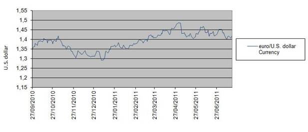
Figure 1: euro/U.S. dollar currency's exchange rate versus time.

 

 

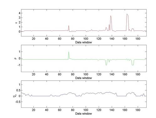
Figure 2: The parameters e, r,  reconstructed from the data of Figure 1 versus time.

 

5. References

[1]  P.S. Hagan, D. Kumar, A.S. Lesniewski, D.E. Woodward, Managing smile risk, Wilmott Magazine, September 2002, (2002), pp. 84-108. Available at http://www.wilmott.com/pdfs/021118_-smile.pdf

 

[2] L. Fatone, F. Mariani, M.C. Recchioni, F. Zirilli, Closed form moment formulae for the lognormal SABR model  and applications to calibration problems, Open Journal of Applied Sciences 3, (2013), pp. 345-359.

 

[3] J.C. Cox, J.E. Ingersoll, S.A. Ross, A theory of the term structure of interest rates, Econometrica 53, (1985), pp. 385-407.

 

[4] F. Black, M. Scholes, The pricing of options and corporate liabilities, Journal of Political Economy, 81, (1973), pp. 637-659

 

[5] L. Fatone, F. Mariani, M.C. Recchioni, F. Zirilli, The use of statistical tests to calibrate the normal SABR model, Journal of Inverse and Ill-Posed Problems 21, (2013), no. 1, pp. 59-84, http://www.econ.univpm.it/recchioni/finance/w15.

 

[6] S. Mergner, Application of State Space Models in Finance, Universitätsverlag Göttingen, Göttingen, Germany, 2004.

 

[7] F. Mariani, G. Pacelli, F. Zirilli, Maximum likelihood estimation of the Heston stochastic volatility model using asset and option prices: an application of nonlinear filtering theory, Optimization Letters, 2, (2008), no. 2, pp. 177-222, http://www.econ.univpm.it/pacelli/mariani/finance/w1.

 

[8] L. Fatone, F. Mariani, M.C. Recchioni, F. Zirilli, Maximum likelihood estimation of the parameters of a system of stochastic differential equations that models the returns of the index of some classes of hedge funds, Journal of Inverse and Ill-Posed Problems, 15, (2007), no. 5, pp. 329-362, http://www.econ.univpm.it/recchioni/finance/w5.

 

[9] L. Fatone, F. Mariani, M.C. Recchioni, F. Zirilli, Some explicitly solvable SABR and multiscale SABR models: option pricing and calibration, Journal of Mathematical Finance, 3, (2013), pp. 10-32,  http://www.econ.univpm.it/recchioni/finance/w14.

 

[10] A. Erdelyi, W. Magnus, F. Oberhettinger, F.G. Tricomi, Higher Trascendental Functions, Vol. II, McGraw-Hill Book Company, New York, U.S.A., 1953.

 

[11] J. Hull, A. White, The pricing of options on assets with stochastic volatilities, The Journal of Finance, 42, (1987), pp. 281-300.

 

[12] B.A. Surya, Two-dimensional Hull-White model for stochastic volatility and its nonlinear filtering estimation, in Procedia Computer Science, 4, (2011), pp. 1431-1440.

 

[13] P. Wilmott, Paul Wilmott Introduces Quantitative Finance, 2, Wiley Desktop Editions, Chichester, West Sussex, England, 2007.