A
trading execution model based on mean field games and optimal control
Lorella Fatone, Francesca Mariani, Maria Cristina Recchioni, Francesco
Zirilli
In [2] we present a trading execution model
that describes the behaviour of a big trader and of a
multitude of retail traders operating on the shares of a risky asset. The
retail traders are modeled as a population of “conservative'” investors
that: i)
behave in a similar way, ii) try to avoid abrupt changes in their
trading strategies, iii) want to limit the risk due to the fact of having open
positions on the asset shares, iv) in the long run want to have a given
position on the asset shares. The big trader wants to maximize the revenue
resulting from the action of buying or selling a (large) block of asset shares
in a given time interval. The behaviour of the retail
traders and of the big trader is modeled using respectively a mean field game
model and an optimal control problem. These models are coupled by the asset
share price dynamic equation. In particular this equation describes how the
asset shares price depends from the trading activity of the retail traders and
of the big trader. The trading execution strategy adopted by the retail traders
is obtained solving the mean field game model. The knowledge of this strategy
is necessary to formulate the optimal control problem that determines the
strategy adopted by the big trader. The mathematical models considered are
solved using the dynamic programming principle. Under some hypotheses the
solution of the mean field game model is reduced to the solution of a
(constrained) two point boundary value problem for a system of six Riccati ordinary differential equations. The optimal
control problem associated to the big trader is a linear quadratic control
problem. Under some hypotheses an explicit formula for the optimal trading
execution strategy of the big trader is deduced. A numerical study of the
trading execution model proposed is presented. The trading execution strategies
obtained with the model developed in [2] and those obtained using alternative
models are compared. This comparison confirms the quality of the model
presented. A general reference to the
work of the authors and of their coauthors in mathematical finance is the
website: http://www.econ.univpm.it/recchioni/finance.
Keywords: mean field game; optimal control; trading
execution strategy.
Content
1. The model
2. The solution
3. Numerical experiments (animation 1, animation 2, animation 3, interactive application, app)
4. References
1.The model
In [2] we consider a market
where a big trader and a multitude of
retail traders operate on the shares of a risky asset.
The big trader want to
maximize the expected (total) revenue resulting from the action of selling a
(large) number of shares of the risky asset in a given time interval (liquidation
problem). The analysis developed to study the liquidation problem can be easily
extended to the study of the problem posed by the execution of a buying order.
The retail traders are
conservative investors that belong to a population of individuals that:
·
behave in a similar way,
·
try to avoid abrupt changes
in their trading strategies,
·
want to limit the risk due
to the fact of having open positions on the asset shares,
·
in the long run want to
have a given position on the asset shares.
The behaviour
of the big trader is modeled using an optimal control problem.
The behaviour
of the retail traders is modeled using a mean field game model [4]. This means
that the behaviour of the retail traders is studied
in the “mean field approximation”. The (time) dynamics of the
trading positions of the retail
traders is substituted with a “mean dynamics” that describes the behaviour of the trading position of a “mean retail
trader”. We recall that the mean field approximation has been introduced
in statistical mechanics to study systems of interacting particles and that has
been used in the social sciences to describe multitudes of “intelligent agents”.
The mathematical models
that describe the big trader and the retail traders are coupled through the
asset price dynamic equation.
The retail traders
model
Let:
·
R be the set of real numbers,
·
T1ÎR be a positive number that represents the time
horizon of the mean field game model that describes the retail traders. This
means that the model that describes
the retail traders is solved in the time interval [0,T1],
·
xt, tÎ[0,T1], be a real
stochastic process that represents the number of shares of the risky asset held
by the retail traders as a function of the time t, tÎ[0,T1]. The variable
xt is called trading
execution strategy or trading position of the retail traders at time t, tÎ[0,T1]. Recall that the variable xt, tÎ[0,T1], describes the retail traders in the mean
field approximation. Positive values of xt, tÎ[0,T1], mean that the retail traders have a long
position on the asset shares, negative values of xt, tÎ[0,T1], mean that the retail traders have a
short position on the asset shares,
·
![]() be a continuous function that represents the
trading rate of the retail traders,
be a continuous function that represents the
trading rate of the retail traders,
·
m(t,x), xÎR, tÎ[0,T1], be the probability density function of the random
variable xt, tÎ[0,T1],
·
σ
be a (non zero) real constant,
·
Wt, ![]() , be a standard Wiener process such
that W0=0 and dWt,
, be a standard Wiener process such
that W0=0 and dWt, ![]() , be its stochastic differential.
, be its stochastic differential.
We assume that the trading execution strategy
of the retail traders xt, tÎ[0,T1], is
solution of the following stochastic differential equation:
![]() (1)
(1)
with
initial condition:
![]() (2)
(2)
where ![]() is a known random variable whose
probability density function is denoted with m0(x), xÎR. The probability density function of xt is denoted by m(t,x), xÎR, tÎ[0,T1].
is a known random variable whose
probability density function is denoted with m0(x), xÎR. The probability density function of xt is denoted by m(t,x), xÎR, tÎ[0,T1].
Equation
(1) is the mean field equation that describes the “mean dynamics”
of the trading position of the “mean retail trader”.
Note that in (1) the function ![]() is not a known coefficient. The function
is not a known coefficient. The function ![]() is the control variable that must be
determined solving the mean field game model.
is the control variable that must be
determined solving the mean field game model.
Let E(![]() denote the expected value of
denote the expected value of ![]() ,
A1 be
the set of the square integrable processes on [0,T1]
, and λ, θ, a be parameters such that λ>0, θ≥0 and
aÎR.
,
A1 be
the set of the square integrable processes on [0,T1]
, and λ, θ, a be parameters such that λ>0, θ≥0 and
aÎR.
The retail traders adopt the trading execution
strategy whose rate ![]() =
=![]() t=
t=![]() (t,xt), tÎ[0,T1],
solves the following problem:
(t,xt), tÎ[0,T1],
solves the following problem:
![]()
![]() (3)
(3)
where:
![]() (4)
(4)
subject to
the constraints (1), (2).
The model
(3), (4), (1), (2) is the mean field game model used to describe the behaviour of the retail traders.
The big trader model and the asset share price
dynamic equation
Let:
·
T2ÎR be a positive number such that T2≤T1, T2 is the time horizon of the
liquidation problem. This means that the selling order must be executed in the
time interval [0,T2],
·
Y>0
be a positive integer that represents the number of asset shares that must be
sold in the time interval [0,T2],
·
β:[0,T2]
× R → R be a continuous function that
represents the trading rate of the big trader,
·
yt, tÎ[0,T2], be a real
function that represents the number of asset shares of the risky asset held by
the big trader as a function of the time t, tÎ[0,T2].
The variable yt, tÎ[0,T2], is called trading execution strategy of the big
trader.
The liquidation problem of the big trader
consists in determining how to execute the order of selling Y asset shares in
the time interval [0,T2] in order to maximize the expected (total)
revenue resulting from the sale.
We assume that yt, tÎ[0,T2], is solution of
the following differential equation:
![]() (5)
(5)
with
initial condition:
![]() = Y,
(6)
= Y,
(6)
and final
condition:
![]() (7)
(7)
The function βt= β(t,yt), tÎ[0,T2], is the control
variable of the control problem that defines the behaviour
of the big trader.
Note that the differential equation (5) is the
equation used in similar circumstances by Almgren
[1].
The asset price dynamic equation of the model
presented in [2] is a simple generalization of the asset share price dynamic
equation used by Almgren in [1].
Let:
·
![]() be a stochastic process that
represents the price of the asset share “in absence of trading”, we
assume that d
be a stochastic process that
represents the price of the asset share “in absence of trading”, we
assume that d![]() = εdBt,
= εdBt, ![]() [0,T2], where ε>0 is a real parameter
and Bt,
[0,T2], where ε>0 is a real parameter
and Bt, ![]() [0,T2], is a standard
Wiener process, such that B0=0 and dBt
is its stochastic differential. The Wiener processes Wt,
Zt and Bt,
[0,T2], is a standard
Wiener process, such that B0=0 and dBt
is its stochastic differential. The Wiener processes Wt,
Zt and Bt,
![]() [0,T2], are assumed to be independent.
[0,T2], are assumed to be independent.
·
![]()
![]() ζ2
be nonnegative
constants.
ζ2
be nonnegative
constants.
Let St be the asset share
price at time t, ![]() [0,T2], we assume that St,
[0,T2], we assume that St, ![]() [0,T2], is a real
stochastic process defined as follows:
[0,T2], is a real
stochastic process defined as follows:
St = ![]() +
+ ![]() Mt +
Mt + ![]() βt + ζ2(Y-yt), tÎ[0,T2],
(8)
βt + ζ2(Y-yt), tÎ[0,T2],
(8)![]()
![]() given,
(9)
given,
(9)
where Mt = E(α(t,xt)) = E(αt) = ![]() , t
, t![]() [0,T1], βt = β(t,yt), t
[0,T1], βt = β(t,yt), t![]() [0,T1], and we assume that
[0,T1], and we assume that ![]() is a positive random variable
concentrated in a point.
is a positive random variable
concentrated in a point.
Equation (9) is the asset price dynamics
equation.
Note that the
asset price dynamic equation (9) allows negative asset share prices. The same
is true for the asset share price dynamic equation used by Almgren
in [1].
Let A2 be the set of the square integrable processes on [0,T2]. The problem of finding the optimal
trading execution strategy for the big trader consists in solving the following
optimal control problem:
![]() (10)
(10)
where:
V(β) = ![]() , β
, β![]() A2,
(11)
A2,
(11)
subject to
the constraints (5), (6), (7).
The problem (10),
(11), (5), (6), (7), (8), (9) is a linear quadratic optimal control
problem. The function V(β),
β![]() A2 is the expected final revenue resulting
from the liquidation order when the trading execution strategy yt, tÎ[0,T2], determined by β through (5), (6), (7) is adopted.
A2 is the expected final revenue resulting
from the liquidation order when the trading execution strategy yt, tÎ[0,T2], determined by β through (5), (6), (7) is adopted.
2.The solution of the
model
Let N(∙,+)
be the normal probability distribution of mean ∙ and standard deviation +
and let ξ be a random
variable. The notation ξ![]() N(∙,+) means that ξ is a
normal random variable distributed
N(∙,+). Using the ideas of Kalman [3]
under some hypotheses we reduce the solution of the mean field game model (3),
(4), (1), (2) and of the optimal control problem (10), (11), (5), (6), (7),
(8), (9) to the solution of two systems of Riccati
ordinary differential equations (see [2] for more details).
N(∙,+) means that ξ is a
normal random variable distributed
N(∙,+). Using the ideas of Kalman [3]
under some hypotheses we reduce the solution of the mean field game model (3),
(4), (1), (2) and of the optimal control problem (10), (11), (5), (6), (7),
(8), (9) to the solution of two systems of Riccati
ordinary differential equations (see [2] for more details).
In particular in [2] under the hypotheses that: there
exist μ0,
ψ0![]() , ψ0>0, such that
, ψ0>0, such that ![]() N(μ0, ψ0)
we show that
N(μ0, ψ0)
we show that ![]() N(μt,
ψt), tÎ[0,T1], where
N(μt,
ψt), tÎ[0,T1], where ![]() , tÎ[0,T1],
is the solution of the mean field game model (4), (3), (2), (1) and μt, ψt,
tÎ[0,T1], are determined from the
solution of a system of six Riccati ordinary
differential equations.
, tÎ[0,T1],
is the solution of the mean field game model (4), (3), (2), (1) and μt, ψt,
tÎ[0,T1], are determined from the
solution of a system of six Riccati ordinary
differential equations.
Moreover
in [2] when ![]() tÎ[0,T1],
we derive explicit
formulae for Mt, μt, t
tÎ[0,T1],
we derive explicit
formulae for Mt, μt, t![]() [0,T1], these formulae
are substituted in the asset share price dynamic equation (8) in
order to solve the optimal control problem (10), (11), (5), (6), (7), (8), (9).
In [2] we show that the corresponding optimal trading execution strategy of the
big trader yt=
[0,T1], these formulae
are substituted in the asset share price dynamic equation (8) in
order to solve the optimal control problem (10), (11), (5), (6), (7), (8), (9).
In [2] we show that the corresponding optimal trading execution strategy of the
big trader yt=![]() , tÎ[0,T2], solution of the
problem (10), (11), (5), (6), (7), (8), (9) is the solution of the following
differential equation:
, tÎ[0,T2], solution of the
problem (10), (11), (5), (6), (7), (8), (9) is the solution of the following
differential equation:
![]() (12)
(12)
with
initial condition:
![]() (13)
(13)
Recall
that since the formulae for Mt, μt,
tÎ[0,T2], deduced in [2] have been
obtained under the assumption ![]() N(μ0, ψ0)
also the formula for
N(μ0, ψ0)
also the formula for ![]() t
t![]() [0,T2], deduced in [2]
from (12), (13) holds under the assumption
[0,T2], deduced in [2]
from (12), (13) holds under the assumption ![]() N(μ0, ψ0).
N(μ0, ψ0).
3. Numerical experiments
Let us study the trading execution model
presented in Sections 1 and 2 via numerical simulation. In particular we consider
a liquidation order and in a test case we compare the value of the expected
total revenue of the big trader (11) associated to the optimal trading
execution strategy (12), (13) that we have found as solution of our model with
the expected total revenue of two alternative trading execution strategies.
We assume that:
·
the
number of asset shares held by the big trader at time t=0 is Y=2,
·
the
final time within which the sale must be completed is T2=0.6,
·
the
remaining parameters of the models of Section 1 and 2 have the following
values: T1=1, ![]() =10,
=10, ![]() =1, ζ2=0, λ=0.5, σ=0.8, μ0=10,
ψ0=0.5 and a=-50, θ=1.
=1, ζ2=0, λ=0.5, σ=0.8, μ0=10,
ψ0=0.5 and a=-50, θ=1.
Note that the choice:
·
μ0=10
implies that the retail traders are buyers at time t=0,
·
a=-50
implies that the retail traders are sellers at time T1.
With the
previous choices the optimal trading execution strategy of the big trader
determined by our model from being a concave function of t when t is close to
zero becomes a convex function of t when t is close to T2.
To fix the ideas we consider three trading
execution strategies (Strategy 1, Strategy 2, Strategy 3) that are shown in the
three animations that follow.
1.
In
animation 1 we show the optimal trading execution strategy of the big trader yt=![]() , tÎ[0,T2],
obtained as solution of the model presented in Sections 1 and 2 defined by
(12), (13) and in [2]. This is Strategy 1.
, tÎ[0,T2],
obtained as solution of the model presented in Sections 1 and 2 defined by
(12), (13) and in [2]. This is Strategy 1.
2.
In
animation 2 we show the trading execution strategy of the big trader defined as
follows:
![]() (14)
(14)
where ![]() , tÎ[0,T2],
is the optimal trading execution strategy shown in animation 1. This is
Strategy 2.
, tÎ[0,T2],
is the optimal trading execution strategy shown in animation 1. This is
Strategy 2.
3.
In
animation 3 we show the
optimal trading execution strategy of the big trader found in the “same
circumstances” using Almgren’s model [1]
that consists in selling with constant rate in the time interval [0,T2],
that is:
![]() (15)
(15)
This is Strategy
3.
Note that
Strategy 1 (see animation 1) makes use of
short selling (i.e.: yt becomes
negative for some values of tÎ[0,T2]). Strategy 2 and Strategy 3 do not use short selling.
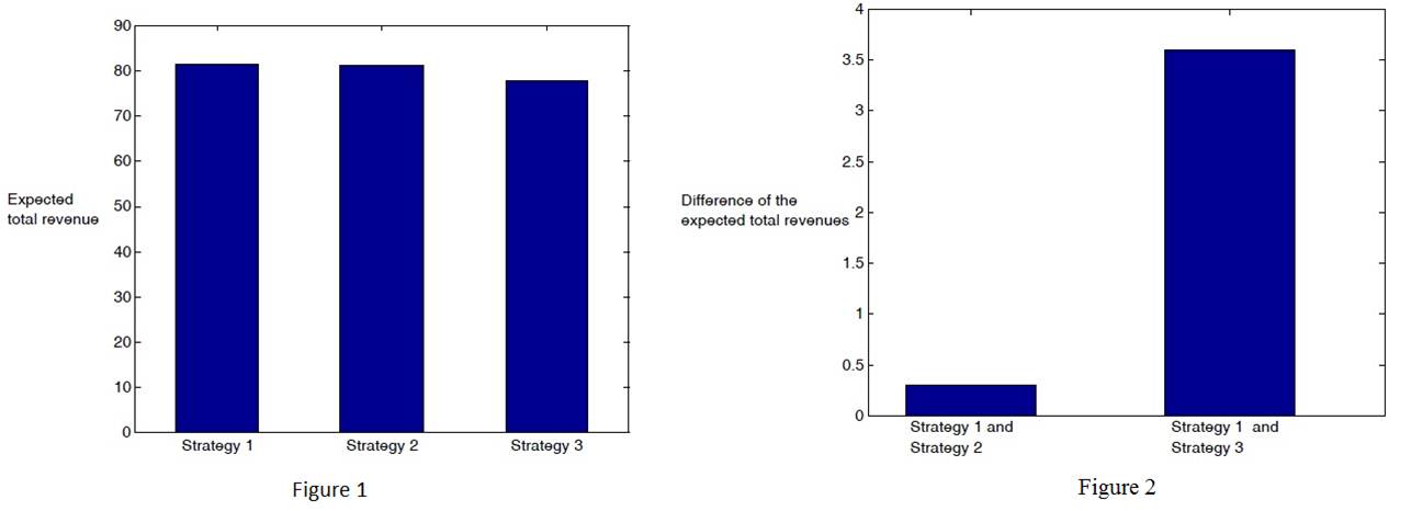
In Figure 1 we compare the values of the
expected total revenue (11) associated to the trading execution Strategies 1,
2, 3. As it should be the expected total revenue associated to the optimal trading
execution strategy, Strategy 1, is greater than the expected total revenues
associated to Strategy 2 and Strategy 3.
In Figure 2 we show the difference between the
expected total revenues associated to Strategy 1 and Strategy 2 and the
difference between the expected total revenues associated to Strategy 1 and
Strategy 3.
Finally an interactive application and an app
are presented. The interactive application computes and draws on a graph the
optimal trading execution strategy of the big trader, the mean value of the
trading execution strategy of the retail traders and the asset price dynamics.
In the interactive application the user must assign the values of some of the model
parameters. To facilitate the use of the interactive
application a set of default values of these parameters is given. The
remaining parameters of the models involved in the numerical simulation are
chosen as follows: ![]() =10,
=10, ![]() =1, ζ2=0, λ=0.5, σ=0.8, ψ0=0.5
and θ=1. Recall that the random variable
=1, ζ2=0, λ=0.5, σ=0.8, ψ0=0.5
and θ=1. Recall that the random variable ![]() that appears in (9) is chosen to be a
random variable concentrated in the point
that appears in (9) is chosen to be a
random variable concentrated in the point ![]() (assigned by the user) with probability
one.
(assigned by the user) with probability
one.
The interactive application has
been transformed in an app. The app runs on devices
based on the Android software system including smart phones and tablets.
App
4. References
[1] R. Almgren (2003). Optimal execution with nonlinear impact functions and trading enhanced risk. Applied Mathematical Finance 10(1), 1-18.
[2] L. Fatone, F. Mariani, M.C. Recchioni, F. Zirilli (2014). A trading execution model based on
mean field games and optimal control. Applied
Mathematics 5(19), 3091-3116.
[3] R. E. Kalman
(1960). A new approach to linear filtering and prediction problems. Journal of Basic Engineering 82 (1),
35-45.
[4] J. M. Lasry,
P. L. Lions (2007). Mean field games. Japanese
Journal of Mathematics 2(1), 239-260.
[5] D. Revuz, M. Yor (1999). Continuous
Martingales and Brownian Motion. Springer-Verlag,
New York.
|
Entry n. |
1 |