PAPER:
The Barone-Adesi Whaley formula to price American options revisited
Lorella Fatone,
Francesca Mariani, Maria
Cristina Recchioni, Francesco
Zirilli
- Abstract
- A perturbation expansion to solve the
American option pricing problem
- Some numerical experiments (Movie 1, Movie 2)
- An
interactive
application and an app
- The importance of the accuracy of the free
boundary approximation: a numerical experiment
- References
.
In [4] we present a method
to solve the American option pricing
problem in the Black Scholes framework that generalizes the Barone-Adesi, Whaley method [1]. An
auxiliary parameter is introduced in the American option pricing problem. Power series expansions in this parameter of
the option price and of the corresponding free boundary are derived. These
series expansions have the Baroni-Adesi, Whaley formula as zero-th order term.
The coefficients of the option price series are explicit formulae. The partial
sums of the free boundary series are
determined numerically as solutions of
nonlinear equations that depend
from the time variable as a parameter.
Numerical experiments on test problems suggest that the series
expansions derived are convergent. The evaluation on a grid of values of the
independent variables of the truncated
series expansions is easily
parallelizable. The cost of computing
the n-th order approximations of the series expansions is approximately
proportional to n as n goes to infinity. The results obtained on a set of test
problems with the first and second order
approximations deduced from the series expansions of the option prices
and of the corresponding free
boundaries outperform in accuracy and/or in computational cost the results
obtained with alternative methods ([1], [2], [3]). In
particular when we consider options with
maturity time between three and ten years
and positive cost of carrying parameter (i.e. when the continuous
dividend yield is smaller than the risk free interest rate) the second order approximation of the free
boundary obtained from the series expansions improves substantially the free boundary
obtained with the Barone-Adesi, Whaley formula [1].
This website contains
material including animations, an
interactive application and an app that helps the understanding of [4]. A general reference to the work of the authors
and of their coauthors in mathematical finance is the website:
http://www.econ.univpm.it/recchioni/finance.
2. A perturbation
expansion to solve the American option pricing problem
We present a method
to solve the American option pricing problem that generalizes the Barone-Adesi,
Whaley method [1]. To fix the ideas we consider options on
commodities as done in [1]. Let t be a real variable that denotes
time and St, t>0, be a real stochastic process that models the
commodity price. Under the risk neutral measure we assume that St,
t>0, satisfies the following stochastic differential equation:
|
dSt=b St dt+s
St dzt , t>0, |
(1)
where b, s are
real parameters, zt, t>0, is a standard Wiener process such that
z0=0 and dzt is its
stochastic differential. The parameter s>0
is the volatility or instantaneous standard deviation and the parameter b is
the cost of carrying. In the most common situations we have b=r-d where
r>0 is the risk free interest rate and d>0 is the continuous dividend
yield. Equation (1) is called Black Scholes asset price dynamic equation.
We study the American
call option pricing problem. The results obtained for the American call option pricing
problem are easily extended to the American put option pricing problem. Let us consider an American call option with maturity time
T>0 and strike price E>0 on a commodity whose price St, t>0,
satisfies (1). We denote with t=T-t, 0 £ t £ T, the
time to maturity, with S the commodity price. Let CA(S,t),
0<S<S* (t), 0 £ t £ T, and
S* (t),
0<t<T, be
respectively the price and the free boundary of the option studied. The American call option
pricing problem written in the independent variables S, t for the unknown
functions CA, S* is
given by:
 (2)
(2)
and initial condition
Following Barone-Adesi and Whaley [1]
we look for a solution of problem (2), (3) , (4), (5), (6) given
by the sum of the price CE(S,t), S>0, 0<t<T,
of the European call option having strike price E, maturity time T and
parameters of the Black Scholes asset
price dynamic equation b and s and of a quantity e(S,t), 0<S<Sf(t),
0<t<T,
called early exercise premium. Moreover we assume that the early exercise premium e is written as follows (see [1]):
where
K(t)=![]() , 0<t<T, and f is an auxiliary function to be
determined. That is we assume that the American call option price is given by:
, 0<t<T, and f is an auxiliary function to be
determined. That is we assume that the American call option price is given by:
Note
that the price CE is defined for S>0, 0<t<T, has a
closed form expression known as Black Scholes formula and satisfies (2), (3), (6). From K(0)=0 and the fact that CE satisfies
(6) it follows that
when f is well behaved in t=0 the
option price CA given
by (8) satisfies (6). Substituting (8) in (2), (3), (4), (5) and using the fact that CE satisfies (2), (3), (6) we obtain the
following problem for the unknown functions f, S* :
 (9)
(9)
![]() (10)
(10)
![]() (11)
(11)
 (12)
(12)
where M=2r/s2 and N=2b/s2 . Note
that K=K(t),
0<t<T,
and that in the formulation of problem (9), (10), (11), (12) we use both K and t as variables.
In [1] Barone-Adesi and Whaley dropped the term (1-K)M(¶ f/¶ K) in (9) and solved the remaining problem. The idea of dropping the term (1-K)M(¶ f/¶ K) in (9) is ingenious and fruitful. In fact the term (1-K)M(¶ f/¶ K) tends to zero when t goes to zero and
when t goes to
T and T goes to infinity, this implies that the Barone-Adesi, Whaley formula is
accurate when we consider options with
short or with long maturity time.
The revisited Barone-Adesi, Whaley formula presented in [4]
is based on the introduction of an auxiliary parameter in the right hand side
of (9) and in the use of power series expansions in this parameter to
approximate the price and the free boundary of the American option pricing
problem considered. The zero-th order terms of these expansions are the
Barone-Adesi, Whaley formula. Specifically equation
(9) is replaced with
the following equation:
 (13)
(13)
where e is the
announced auxiliary parameter. We study
problem (13), (10), (11), (12) and we consider the following series expansions
in powers of e of the function f and of the corresponding
free boundary S* :
![]() (14)
(14)
![]() (15)
(15)
|
|
|
where the
functions fn, Sn* , n=0,1,¼, are
independent of e. In [4] using (13), (10), (11),
(12) we determine the coefficients of the option price series expansion (14)
and the partial sums of the free boundary series expansion (15). The
coefficients of the option price series expansion are explicit formulae that
contain the free boundary. The partial sums of the free boundary series
expansion are determined numerically solving nonlinear equations that contain
the time to maturity t as a parameter, 0≤t ≤T. Let f be well behaved in t =0.
In this case problem (13), (10), (11), (12) when e=1 is
equivalent to the American call option pricing problem (2), (3), (4), (5), (6), when e=0 is
the problem solved by Barone-Adesi, Whaley in [1] and
when e à 0+ is a singular perturbation problem. In
fact note that when e=0
the higher order derivative with respect to K contained in (13) is multiplied
by zero. This fact suggests that when eà 0+ an expansion of fe, Se* in powers of e with base point e=0 does not hold uniformly in K
and S for 0<K< 1-e-rT ,
0<S< However
in finance the solution of problem (13), (10), (11), (12) is relevant
only when e=1. The
behaviour of the solution of problem (13), (10), (11), (12) when eà 0+ has no interest in finance. We avoid
the study of problem (13), (10), (11), (12) when eà 0+ . In fact in [4] we impose to the truncated series
expansions (14), (15) the boundary conditions (11) , (12) in e=1 instead of imposing them in e=0 order by order in perturbation
theory to the inner and outer expansions of the matched asymptotic expansion
method (see [4]). Note that the series expansions (14) , (15) are a kind of
outer expansion of the solution of problem (13), (10), (11),
(12). The functions 3. Some numerical experiments (movie
1, movie 2)
Let
us present some numerical results obtained on a set of test problems with the
solution method sketched in Section 2 (see [4]). We use the
trinomial tree method [5] with nT = 1000 time steps to compute the ``true
value" of the option prices considered in our experiments. The choice nT = 1000 guarantees four correct
significant digits in the option prices computed in the experiments. For
American call options the ``true value" of the free boundaries
considered is computed solving
numerically the integral equation satisfied by the free boundary presented in
[3], [6] and recalled in [4]. We begin our
numerical experiments studying some test problems taken from [1]
Section C.4. These test problems consider options on long-term U.S. Treasury
bonds (time to maturity up to three years) and long term care insurance
inflation options (time to maturity up to ten years and beyond). In the first
experiment we use the Black Scholes parameter values of [1]
Table V. That is we consider the following three sets of parameter values: r
= 0.08, s = 0.2, and b = -0.04, or b = 0.0 or b =
0.04. For each set of Black Scholes parameter values we consider three call
options with strike price E = 100 and maturity time T = 3, or T = 5, or T =
10. The time T is expressed in years. Table 1 shows the free boundary approximations
of the American call option pricing problems specified above when t = T =
3,5,10. From left to right Table 1 shows the free boundary S*(T)
computed solving iteratively the discretized version of the integral equation
presented in [6] (i.e. S*(T)
is the ``true free boundary" used as benchmark) and the approximations When r=0.08, s = 0.2, b = -0.04, and t = T Table 2 shows the asset price S, the European call option
price CE obtained
evaluating the Black Scholes formula in S, t, and the
approximations of the American call option price in S, t obtained using the
trinomial method CT (i.e. CT is the ``true value" of the option price used
as benchmark), the Barone-Adesi, Whaley formula CBW and the n-th order approximation CA,n,e = 1, n =
1,2, derived from (14), (15), (8) using the method presented in [4]. Furthermore we show the relative errors that follows: reBW(S,T)
= |CBW(S,T)-CT(S,T)|/CT(S,T),
(16) and reCn,e = 1(S,T) = |CA,n,e = 1(S,T)-CT(S,T)|/CT(S,T), n
= 1,2. (17) Table
1: Approximations of the free boundary of an American call option with
intermediate maturity T and strike price E = 100.
Table
2: Approximations of the price of an American call option with intermediate
maturity T, strike price E = 100 and negative cost of carrying.
Note
that Tables 1 and 2 show that increasing the approximation order of the
solution of the American call option pricing problem obtained from the
expansions in powers of e (14),
(15) studied in [4] and mentioned in Section 2 (that is increasing n) it is possible to improve substantially the
results obtained with the Barone-Adesi, Whaley formula (i.e. the result
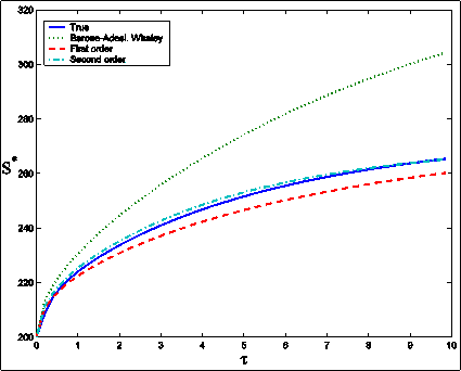
obtained when n = 0). Figure 1 shows the ``true" free boundary,
the Barone-Adesi, Whaley free boundary, the first and the second order
approximations of the free boundary obtained with the expansions (14), (15) developed
in [4] and sketched in Section 2 as a function of t,
0<t<T,
when E = 100, T = 10, r = 0.08, s = 0.2, d = 0.04 (b=r-d). This figure shows that the first order approximation
of the free boundary improves significantly the zero-th order approximation
of the free boundary (i.e. the Barone-Adesi, Whaley free boundary) and that
the second order approximation of the free boundary refines the result
obtained with the first order approximation. Movie 1 shows the ``true" free boundary, the
Barone-Adesi, Whaley free boundary, the first and the second order
approximations of the free boundary obtained with the expansions developed in
[4] and sketched in Section 2 when E = 100, T = 10, r = 0.08, s = 0.2
as a function of the time to maturity t, 0<t<T, for d=r-b, b=bi=-0.06+i0.006, i=0,1,2…20. That is for i=1,2,...,20 the i-th frame of Movie 1 shows the
American call option free boundary as a function of time to maturity t, 0<t<T, T=10, obtained using the
integral equation deduced in [6] called “true
free boundary”, the Barone-Adesi, Whaley formula, and the first
and second order approximations resulting from the truncation of the power series expansions deduced in [4] when b= bi. Movie 1
Figure 1: American call option free
boundary S* as a function of the time to maturity t, 0< t<T, when E = 100, T
= 10, r = 0.08, s = 0.2, b = 0.04:
``true" free boundary (solid line), Barone-Adesi, Whaley free boundary
(dotted line), first order approximation of the free boundary (dashed line),
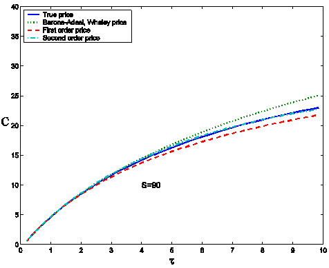
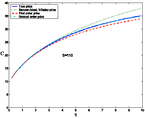
second order approximation of the free boundary (dash-dotted line). Figures 2 (a), 2(b) show the
``true" and the approximated prices of the American call option
corresponding to the free boundaries shown in Figure 1 as a
function of the time to maturity t, 0 £ t £ T,
T=10, when the asset price S takes the values S = 90 (Figure 2 (a))
and S = 110 (Figure 2 (b)). The approximated option prices are
obtained using the zero-th, first and second order approximations obtained
truncating the series expansions deduced in [4] and
sketched in Section 2. Figures 1 and 2 suggest
that the second order corrections of the option price and of the free
boundary are necessary to have satisfactory numerical solutions of the
American call option pricing problem when we consider at time t=0 or at time t close to zero options with
intermediate maturity times (i.e. 3 £ T £ 10). Movie 2 illustrates the relation between the
three approximations mentioned above of the American call option price. In
particular Movie 2 shows the American call option prices as a function of the time to maturity for a
fixed value of the asset price obtained using the trinomial tree method (called
“true price”), the Barone-Adesi,
Whaley formula, and the first and second order approximations resulting from
the truncation of the power series expansions (14), (15) studied in [4]. The parameter
values of the American call option pricing problem considered in Movie 2 are those of Figure 2(a), 2(b), that is
dividend yield d=0.04 (b=r-d=0.04), interest rate r=0.08, volatility s=0.2, asset price
S=90, time to maturity t between 0 and 10
years, strike price E=100.
Figure 2(a)
Figure 2(b) Figure 2: American call option price C as a function of the time to
maturity t for two values
of the asset price S = 90 (a), S = 110 (b), when E = 100, T = 10, r =
0.08, s= 0.2, b = 0.04.
``True" price CT (solid line), Barone-Adesi, Whaley
price CBW (dotted line), first order approximation CA,1,e = 1 of the price (dashed
line), second order approximation CA,2,e = 1 of the price
(dash-dotted line). 4. An interactive application and an app An interactive application
to solve the American option pricing problem with the Barone-Adesi, Whaley
formula and with the first and second order approximations obtained
truncating the series expansions (14), (15) developed in [4]
and sketched in Section 2 is provided. The interactive application takes as
input data the volatility s, the risk free
interest rate r, the dividend yield d, the strike price E, the asset price S, the time to maturity t and the type
(call or put) of the American option considered. The output of the interactive application is the
price and the free boundary of the American option pricing problem corresponding
to the values S and t assigned computed using the Barone-Adesi, Whaley
formula and the first and second order approximations obtained truncating the
series expansions (14), (15). The app is a simple translation of the interactive
application in the Android environment. The appis freely downloadable and runs on devices based on the Android
software system. For example it can be
used on Android smart phones and
tablets. 5. The importance of the accuracy of the free
boundary approximation: a numerical experiment We
present a numerical experiment that shows the relevance of having an accurate
approximation of the free boundary for
the holder of an American option. Let us recall that the values of the parameters
that define the experiment are: E = 100, T = 10, r = 0.08, s = 0.2, d = 0.04, b=r-d=0.04. We consider the American call
option pricing problem corresponding to these parameter values whose free boundary as a function of the time
to maturity is shown in Figure 1. Let
us recall that we work in the Black Scholes framework and that in this
framework we have a market where there are no arbitrage opportunities, no transaction costs and the asset price dynamics
is given (1). We
consider four investors holding the American call option specified above. We
suppose that the first investor knows the “true” value of the free boundary and
that the last three investors know only an approximation of it. That is the
second, third and fourth investor knows, respectively, the zero-th, first and
second order approximations of the free boundary obtained truncating the
series expansions (14), (15) with the method sketched in Section 2. These four
investors sell the option when the underlying asset price reaches the free
boundary known to them and capitalize the revenue of the sale (i.e. the
option price) from the time of the sale up to time T at the risk free
interest rate. Note that these four investors
adopt the decision of selling the option when the underlying asset price
reaches the free boundary, that is they adopt the optimal decision suggested
by the mathematical analysis of the American option pricing problem. More
specifically in the experiment we
simulate 10000 trajectories with a time step Dt=0.001(years) of
the price, St, t=ti=iDt, i=1,2,…,10000,
starting from an initial asset value S0 at t=0 that is smaller
than the “true” free boundary and than the approximated free boundaries known
to the investors considered. Each investor checks at t= ti , i=1,2,…,
10000, whether the simulated asset price is greater than the free boundary
known to him. When this is true for the first time at t=
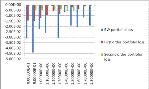
Figure 3:
Percentage of loss rBW=E((Vtrue-VBW )/Vtrue ), r1=E((Vtrue-V1)/Vtrue ) and r2=E((Vtrue-V2 )/Vtrue) of the three holders that know only an approximation of the free
boundary for different values of the moneyness S0/E. Figure 3 shows that the investors that know a
more accurate approximation of the free boundary do better than those that
know a poorer approximation of the free boundary. This effect is more
relevant when options out of the money
(i.e. S0/E<1) and at the money (i.e. S0/E»1) are considered.
6. References
[1] Barone-Adesi, G., Whaley, R.E. (1987). Efficient
analytical approximation of American option values. The Journal of Finance,
Vol. 42(2), 301-320. [2] Ju, N., Zhong, R.
(1999). An approximate formula for
pricing American options. The Journal of Derivatives, Vol. 7(2), 31-40. [3] Little, T., Pant, V., Hou,
C. (2000). A new integral representation of the early exercise boundary for
American put options. Journal of Computational Finance, Vol. 3, 73-96. [4] Fatone, L., Mariani, F., Recchioni,
M.C., Zirilli, F.: The
Barone-Adesi Whaley formula to price
American options revisited, in
preparation. [5] Boyle, P.
(1986). Option Valuation using three-jump process. International Options
Journal, Vol. 3, 7-12. [6] Secovic, D. (2001). Analysis of the free
boundary for the pricing of an American call option. European Journal of
Applied Mathematics, Vol. 12(1), 25 - 37. |
|||||||||||||||||||||||||||||||||||||||||||||||||||||||||||||||||||||||||||||||||||||||||||||||||||||||||||||||||||||||||||||||||||||||||||||||||||||||||||||||||||||||||||||||||||||||||||||||||||||||||||||||||||||||||||||||||||||||||||||||||||||||||||||||||||||||||||||||||||||||||||||||||||||||||||||||||||||||||||||||
|
|||||||||||||||||||||||||||||||||||||||||||||||||||||||||||||||||||||||||||||||||||||||||||||||||||||||||||||||||||||||||||||||||||||||||||||||||||||||||||||||||||||||||||||||||||||||||||||||||||||||||||||||||||||||||||||||||||||||||||||||||||||||||||||||||||||||||||||||||||||||||||||||||||||||||||||||||||||||||||||||||


