PAPER:

Determining a stable relationship between hedge fund index HFRI-Equity and S&P 500 behaviour, using filtering and maximum likelihood

Paolo Capelli, Francesca Mariani, Maria Cristina Recchioni,

Fabio Spinelli, Francesco Zirilli

1. Abstract

2. Introduction

3. The calibration procedure and the formulae used to forecast the log-returns

4. Analysis of the S&P 500 and HRFI Equity indices (digital movies)

5. References

Warning: If your browser does not allow you to see the content of this website click here to download a word file that reproduces the material contained here.

1. Abstract

We test the ability of a stochastic differential model proposed in [5] of forecasting the returns of a long-short equity hedge fund index and of a market index, that is of the HFRI-Equity index and of the S&P 500 index respectively. The model is based on the assumptions that the value of the variation of the log-return of the hedge fund index (HFRI Equity) is proportional up to an additive stochastic error to the value of the variation of the log-return of a market index (S&P 500) and that the log-return of the market index can be satisfactorily modeled using the Heston stochastic volatility model. The model consists in a system of three stochastic differential equations, two of them are the Heston stochastic volatility model and the third one is the equation that models the behaviour of the hedge fund index and its relation with the market index. The model is calibrated on observed data using a method based on filtering and maximum likelihood proposed in [9] and further developed in [4], [5], [6]. The data observed and analyzed go from January 1990 to June 2007, and are monthly data. For each observation time they consist in the value at the observation time of the log-returns of the HFRI-Equity and of the S&P 500 indices. The calibration procedure uses appropriate subsets of the data, that is the data observed in a six months time period. The values of the HFRI-Equity and of the S&P 500 indices log-returns forecasted by the calibrated models are compared to the values of the observed indices log-returns. The result of the comparison is very satisfactory. This website contains some auxiliary material that helps the understanding of [4]. A more general reference to the work of some of the authors and of their coauthors in mathematical finance is the website: http://www.econ.univpm.it/recchioni/finance.

2.  Introduction

We test on real data the model proposed in [4], [5] that describes the dynamics of the index of some classes of hedge funds and of a market index. Let us recall the model proposed. We denote with R and R⁺ the set of real numbers and of positive real numbers respectively, with t the time variable, and with (x_t,z_t,v_t), t > 0, a stochastic process, we will interpret x_t, t > 0, as the log-return of a market index, z_t, t > 0, as the log-return of the index of a class of hedge funds and v_t, t > 0, as the stochastic variance of the market index. We consider the S&P 500 index as market index and the HFRI-Equity hedge fund index as index of a class of hedge funds, that is the class of ``long-short equity" hedge funds. The model proposed in [4], [5] can be used with several other choices for the meaning of the indices. In [4], [5] the dynamics of the stochastic process (x_t,z_t,v_t), t > 0, is modeled by the following system of stochastic differential equations:

with initial condition:

where , b, g, c, q, e are constants, , , , t ³ 0, are standard Wiener processes such that W₀¹=W₀²= W₀³ =0, and d, d, d, t>0, are their stochastic differentials. Moreover we assume that:

< dW^1t dW^2t >	=	r1,2 dt,  t > 0,	(7)
< dW^1t dW^3t >	=	r1,3 dt,  t > 0,	(8)
< dW^2t dW^3t >	=	r2,3 dt,  t > 0,	(9)

where < · > denotes the expected value of ·, and the quantities r_1,2, r_1,3, r_2,3 Î [-1,1] are constants known as correlation coefficients. We note that the autocorrelation coefficients of dWⁱ_t, t>0, i = 1,2,3 are equal to one.

Equations (1), (3) are the well known Heston stochastic volatility model [8]. This model was introduced with the aim of overcoming some limitations of the Black Scholes model [3] that are pointed out by market data such as, for example, the assumption of constant volatility. Let S_t, t > 0, be the price at time t of an asset, the Heston model (1), (3) describes satisfactorily the dynamics of the log-return x_t = log(S_t/S₀), t > 0, of the asset and of its stochastic variance v_t, t > 0. Note that x₀ = log1 = 0 = and that since z_t, t>0, is a log-return a similar statement holds for z₀, that is z₀ = 0 = . A systematic data analysis has shown that the Heston stochastic volatility model is well suited to model the behaviour of several market indices such as, for example, the S&P 500 index, the Dow-Jones Industrials index and the Nasdaq Composite index (see [7]). We note that equation (3) is known as equation of the mean-reverting process with speed c and parameters q and e. The initial stochastic variance is a random variable that we assume to be concentrated in a point, that we continue to denote with , with probability one.

We note that the model (1), (2), (3) introduced in [5] and analyzed on real data in [4] is obtained adding to the Heston stochastic volatility model (1), (3) a third equation, that is equation (2), that describes the behaviour of the log-return of the index of some classes of hedge funds. In fact statistical studies, such as [10], of the time series of the data relative to the log-returns of the indices of several classes of hedge funds have shown that the log-returns of the indices of some classes of hedge funds are related to the log-returns of the S&P 500 index. In particular in [10] some discrete time models are proposed to study nine different classes of hedge funds. The model proposed in [10] to describe the dynamics of the log-return of the index of the “long-short equity” class of hedge funds is based on the assumption that up to a stochastic additive error there exists a kind of direct proportionality between the behaviour of the variation of the log-return of the index of the “long-short equity" class of hedge funds and the variation of the log-return of the S&P500 index. In [10] this assumption is supported by convincing empirical evidence. So that interpreting z_t, t>0, as the log-return at time t of an index of the “long-short equity" class of hedge funds, that is the HFRI-Equity index, x_t, t>0, as the log-return at time t of the S& P500 index and v_t, t>0, as the stochastic variance of x_t, t>0, the system of stochastic differential equations (1), (2), (3) obtained coupling the Heston model (1), (3) with equation (2) can be seen as a reasonable translation in continuous time of the model proposed in [10]. In fact equation (2) states that dz_t is given by the sum of b dx_t and a random disturbance given by gdW_t³.

The calibration problem of model (1), (2), (3) can be stated as follows: given a discrete set of time values t=t_i, i=0,1,…,n, such that t₀=0, t_i<t_i+1, i=0,1,…,n-1, and the observation of the log-returns of the market and of the hedge fund indices, that is the observation of (x_t,z_t), at time t=t_i, i=0,1,…,n, determine the values of the parameters appearing in (1), (2), (3), of the correlation coefficients r_1,2, r_1,3, r_2,3 and of the initial stochastic variance . That is the parameters (including the correlation coefficients) and the unknown initial condition component of model (1), (2), (3) that we want to estimate starting from the observations are: , q, c, e, g, b, r_1,2, r_1,3, r_2,3 and .

Note that the choice t₀=0 corresponds to choosing the origin of the time axis in the first observation time where we choose =(0,0). Note that the origin of the time axis can be moved at our convenience in the time series of the data without changing substantially the problem considered.

In order to study time series of real data the calibration problem of model (1), (2), (3) stated previously has been solved using the approach suggested in [5] based on the methods of filtering and maximum likelihood. This approach was introduced in the context of mathematical finance in [9] and further developed in [5], [6]. Going into details, we suppose that at discrete times 0=t₀<t₁<t₂<…<t_n<t_n+1 =+¥, the log-return of the S&P500 index and the log-return of the HFRI Equity index are observed and let F_t= {(,) : t_i £t}, t>0, be the set of the observations available at time t>0 of the log-returns of the market index x_t and of the log-returns of the index of the hedge funds z_t. We assume that the observations are error free, that is we assume that =, =, i=0,1,…,n. Let be the vector of the model parameters (including the correlation coefficients) and of the initial stochastic variance, where the superscript ^T denotes the transposed operator. We use the notation t₀ =0 and F₀={()}to simplify some of the formulae that follow.

We determine the joint probability density function of having x_t=x, z_t=z and v_t =v at time t>0 conditioned to the observations contained in F_t, t>0, and to the initial condition (6). Note that the initial conditions (4), (5) are already contained in F_t, t>0. This joint probability density function is determined solving a filtering problem that has been presented in [9], [5], [6].

In [5] the calibration problem is translated in a maximum likelihood optimization problem (see Section 3). We apply these methods to analyze real data. In particular we consider the time series of monthly data of the S&P 500 and of the HFRI-Equity indices covering a period of 210 months going from January 31, 1990 to June 30, 2007. The observation times will be denoted with t=, i=1,2,…,210, and we introduce t= corresponding to December 31, 1989. From these data we derive the corresponding time series of the log-returns. We have applied the calibration procedure described above using as data the data contained in a window of six consecutive observation times (that is a window covering the data relative to a period of six months) corresponding to twelve data, that is the window corresponding to the data (,) observed at time t=, i=k, k+1,…,k+5 for some k. Note that in the calibration problems derived from the data time series the origin of the time axis is translated to the first observation time contained in the data window considered. The numerical results obtained considering the data windows associated to the choices k=0,1,…,205 are presented in Section 4 and they show that the solutions of the calibration problems considered are really associated to the data time series, that is they are “stable” when the time window of the data used in the calibration is shifted. In fact as shown in Figures 1, 2, 3 the solution of the calibration problem as a function of the time window of the data used in the calibration can be grouped into three sets associated to the data of three non overlapping time periods and in these three sets the parameters (including the correlation coefficients) and the initial stochastic variance found are approximately constants (see Section 4 for further details). After calibrating the model using the data belonging to a six month window we use the resulting estimate of the parameters and of the initial stochastic variance to forecast the market and the hedge fund indices one, three and six months in the future counting as future the time after the last observation time contained in the data window used in the calibration. The forecasted values of the market and of the hedge fund indices are obtained using some formulae derived in [5] that translate to the case of model (1), (2), (3) standard formulae of filtering theory. We perform this forecasting exercise moving the data window along the data time series step by step, at each step we discard the observations relative to the first observation time of the window and we insert the observations relative to the next observation time after the window, that is in the previous notation we consider the data windows associated to k=0,1,...,205.The quality of these forecasts is established a priori using filtering theory and a posteriori comparing the forecasted values with the historical data. The results obtained suggest that the model proposed describes satisfactorily the data, and that it is able to produce high quality forecasts of the value of the hedge fund index log-return several months in the future. Forecasts of approximately the same quality are obtained for the log-returns of the market index. We remark that the forecasts that are expected to be good a priori on the basis of filtering theory are a posteriori actually better than the average forecast.

3.  The calibration procedure and the formulae used to forecast the log-returns

Let us formulate the calibration problem and let us give some formulae used to forecast the log-returns x_t, z_t and the stochastic variance v_t, t > 0, solution of problem (1), (2), (3), (4), (5), (6). Moreover we give some formulae that can be used to evaluate “a priori” the quality of the forecasted values of the log-returns (and of the stochastic variance) as explained in Section 4.

Let us consider the joint probability density function =(x,z,v,t|F_t, Q), (x,z,v) Î R×R×R⁺, t > 0, of having x_t = x, z_t = z, v_t = v given F_t, t > 0, and Q. Remind that = = 0. The joint probability density function is the solution of a filtering problem, and in [4] , [5] we have shown that the function is given by:

i=0,1,…,n, (10)

where G(x,z,v,t,x¢,z¢,v¢,t¢| Q), (x,z,v), (x¢,z¢,v¢) Î R×R×R⁺, t, t¢ > 0, t-t¢ > 0, is the fundamental solution of the Fokker Planck equation associated to the system of stochastic differential equations (1), (2), (3), and we have for: i = 0:

fi(v; Q) = d,

v Î R^+,

(11)

for i = 1,2,...,n:

(12)

where d(^.) is the Dirac’s delta and denotes the left limit t that goes to t_i.

In order to determine the vector Q we solve the calibration problem, that is we solve the optimization problem:

max Q Î M

F( Q),

(13)

where the log-likelihood function F( Q) is given by:

(14)

and the set of the admissible vectors M is given by:

. (15)

We maximize the function (14) using as optimization method a variable metric steepest ascent method. This method is a kind of steepest ascent method based on an iterative procedure that searches the maximum likelihood estimate Q^*, solution of (13), beginning from an initial guess Q⁰ Î M and that for k = 1,2,¼ generates at step k a feasible point Q^k Î M satisfying the inequality F(Q^k) > F( Q^k-1), that is the objective function is monotonically increasing along the sequence {Q^k}, k = 0,1,¼. In the numerical experience presented in Section 4 in the optimization procedure we use as stopping rule the condition:

where e_tol, k_max are positive constants that will be chosen later.

We note that the log-likelihood function (14) is only one possible choice between many other possibilities and that the constraints contained in (15) that define M express some elementary properties satisfied by model (1), (2), (3).

Given the joint probability density function (x,z,v,t|F_t, Q), (x,z,v) Î R×R×R⁺, t ³ 0, we can forecast the values of the market index log-return, of the hedge fund index log-return x_t, z_t, t > 0, t ¹ t_i, i = 0,1,¼,n, and of the stochastic variance v_t, t > 0, using respectively the mean values _{t| Q}, _{t| Q}, _{t| Q}, t > 0, conditioned to the observations contained in F_t, t > 0, of the random variables x_t, z_t, v_t, t > 0, that is:

(17)

(18)

(19)

Note that in Section 4 we are interested in forecasting x_t, z_t, v_t when t>t_n and that this corresponds to the genuine meaning of the word “forecast”.

As shown in [5] from (10), (12), (17), (18), (19), we have:

Remind that we use the notation t_n+1 = +¥. Note that it is easy to see that, as it should be, we have: , , i = 0,1,¼,n. The quality of the forecasted values depends from the variance of the random variables x_t, z_t, v_t, t>0, conditioned to the observations, that is we can estimate the quality of the estimates (20), (21), (22) computing respectively the quantities:

(23)

(24)

(25)

The estimates (20), (21), (22) are expected to be good, when the variances (23), (24), (25) are small. In [5] some formulae similar to (20), (21), (22) are derived from (23), (24), (25).

4. Analysis of the S&P 500 and HRFI Equity indices

Let us present the results obtained applying the procedure described in the previous Sections to the historical series of 210 monthly data relative to the variation DI_x,i of the S&P 500 index I_x,i, at time t=, i = 1,2,¼,210, and to the variation DI_z,i of the HFRI-Equity index I_z,i, at time t=, i=1,2,…,210 (see formulae (30), (31)). The data cover the period of 210 months going from January 31, 1990 to June 30, 2007. The observation dates t =, i = 1,2,¼, 210 are the last day of the month (i.e. January 31, February 28, March 31, April 30, May 31, June 30, July 31, August 31, September 30, October 31, November 30, December 31) of the period January 1990, June 2007. We have added to these data the observation at date t = corresponding to December 31, 1989. We choose I_x,0=I_z,0=1 and , . First of all we have manipulated the data DI_x,i, DI_z,i, i = 1,2,¼, 210, in order to get the time series of the observed log-return , i = 1,¼, 210, of the S&P 500 index and of the observed log-return , i = 1,¼,210, of the HFRI-Equity index. To visualize and eventually download the data click here Table 1 .

We have used the following recursive formulae to construct the log-returns (i.e. the last two columns of Table 1):

where as mentioned above , correspond to the log-returns at time t = (December 31, 1989) that have been chosen equal to zero.

The indices I_x,0, I_z,0 have been assumed to be equal one and I_x,i, I_z,i, i = 1,2,¼, 210 are related to the monthly log-returns , , i = 1,2,¼,210, defined in (26), (27) by the following formulae:

= logIx,i = log(Ix,i-1(1+DIx,i)),   i = 1,2,¼,210,

(28)

= logIz,i = log(Iz,i-1(1+DIz,i)),   i = 1,2,¼,210,

(29)

that is we have:

Ix,i = Ix,i-1(1+DIx,i),   i = 1,2,¼,210,     Ix,0 = 1,

(30)

Iz,i = Iz,i-1(1+DIz,i),   i = 1,2,¼,210,     Iz,0 = 1.

(31)

We consider a window of six consecutive observation times (that is a window covering a time period of six months) corresponding to twelve data and we move from a window to the next one removing the data relative to the first observation time of the window and adding the data corresponding to the observation time that follows the last observation time of the window. That is the j-th window contains the data ( , ), i = 1,2,¼,6, j = 1,2,¼,206. For each data window we solve the calibration problem (13). We have solved 206 calibration problems. Remind that in the solution of each calibration problem, coherently with the statement of the problem given in the Introduction, we translate appropriately the origin of the time axis.

The data analysis presented investigates the following two problems.

Problem 1: understand if the calibration procedure described in Section 2 to determine the value of the vector Q, that is the maximum likelihood problem (13), gives values of Q that are really associated to the data time series, that is values of Q that are approximately constant when we change the data window used in the calibration. If this is the case the values of Q determined by the calibration procedure are not an artifact of the computational procedure used to determine them. Note that despite the fact that the stochastic variance is the solution of a stochastic differential equation it is reasonable to assume that the stochastic variance is approximately constant over long periods of time and that it changes abruptly from time to time.

Problem 2: evaluate the capability of the models corresponding to the values of Q determined with the calibration procedure of forecasting the values of x_t, z_t in the future, that is of forecasting using the formulae (20), (21) the values x_t, z_t relative to observation times posterior to the observation times contained in the data window used to estimate the vector Q. This capability is evaluated a priori using formulae (23), (24) and established a posteriori comparing the forecasted values with the observations actually made. Note that Problem 2 is considered since Problem 1 is solved positively.

Investigation of Problem 1

As said previously we have solved 206 calibration problems relative to the 206 data windows described above determining 206 values of the vector Q. In the solution of the 206 maximization problems (13) we have chosen the initial guess of the maximization procedure to be always the same vector and in the stopping criterion (16) we have chosen e_tol= 5·10^-4 and k_max = 10000.

Figures 1, 2, 3 show (in ordinate) the components of the vector Q obtained solving the maximum likelihood problem (13) as a function of i (in abscissa), where i is the index value of the last observation time of the data window considered. That is the vector Q obtained using a given data window is associated to the index of the last observation time of the data contained in the window.

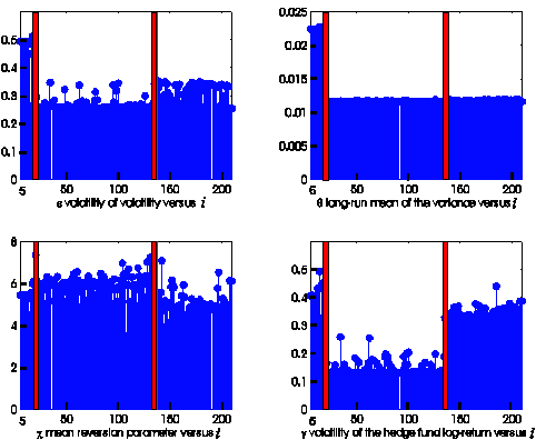
Figure 1: Reconstruction of the parameters e, q, c, g (in ordinate) of the model (1), (2), (3) as a function of the index value of the last observation time contained in the data window considered (in abscissa)

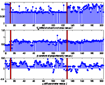
Figure 2: Reconstruction of the initial stochastic variance and of the parameters b, m (in ordinate) of the model (1), (2), (3) as a function of the index value of the last observation time contained in the data window considered (in abscissa)

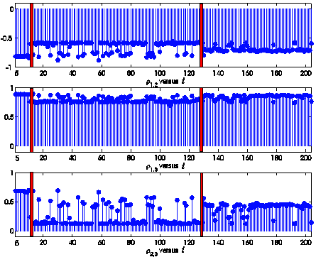
Figure 3: Reconstruction of the correlation coefficients r_1,2, r_1,3, r_2,3 (in ordinate) of the model (1), (2), (3) as a function of the index value of the last observation time contained in the data window considered (in abscissa)

Figures 1, 2 and 3 show that the parameters e, g, the initial stochastic variance and the correlation coefficients r_1,2 and r_2,3 as a function of i are approximately given by piecewise constant functions. In particular two observation times (marked with the red bars in the Figures) where the piecewise constant functions jump are evidenced, the first one is located approximately after the first year of observation (October 31, 1990) and the second one is located approximately after ten years of observations (October 31, 2000). The data analysis carried out and illustrated in Figures 1, 2, 3 shows that the data can be divided into three periods:

• Period 1: this period (from the beginning of the time series up to the first red bar) is very small and covers the period going from December 31, 1989 to October 31, 1990;
• Period 2: this period (between the first and the second red bar) is quite long and covers the period going from November 30, 1990 to October 31, 2000;
• Period 3: this period (after the second red bar until the end of the time series) covers the period going from November 30, 2000 to June 30, 2007.

That is the data analysis carried out solving the 206 calibration problems considered shows that the vectors Q determined by the calibration procedure can be considered approximately constants in each one of the three Periods mentioned above.

Moreover in Figure 3 we can see that the correlation coefficient r_1,3 that measures the correlation between two of the stochastic differentials present in the equations of the log-return of the S&P 500 index and of the log-return of the hedge fund HFRI-Equity index, is almost constant and approximately equal to one over the entire observation period. This fact seems to confirm the validity of model (1), (2), (3) that assumes that the behaviour of the hedge fund HFRI-Equity index depends strongly from the behaviour of the S&P 500 index. Furthermore the fact that the parameter b is substantially constant (exception made when we go from Period 1 to Period 2 where b goes approximately from 0.5 to 0.7) confirms the assumption of the existence of a kind of “proportionality” between the variations of the HFRI-Equity hedge fund index and of the S&P 500 index log-returns.

We can conclude that the data analysis presented shows a convincing evidence of the fact that the values of the vector Q determined by the maximum likelihood procedure (13) are really associated to the data time series and supports some of the assumptions made to build model (1), (2), (3).

Investigation of Problem 2

The second problem addressed in the data analysis is the investigation of the quality of the forecasted values of the log-returns of the indices obtained using model (1), (2), (3) and the values of Q shown in Figures 1, 2, 3 determined solving the calibration problems. That is, we use the values of the vectors Q determined solving the maximum likelihood problems and formulae (20), (21) to forecast the values of the returns x_t and z_t and of the increments of the HFRI-Equity index= , i=5,6,…,210-m, m = 1,2,¼,6, that is one month, two months,... up to six months in the future. Note that here “future” means the time that follows the last observation contained in the data window used to estimate the vector Q.

Let N_tot be a positive integer that denotes the number of forecasted values m months in the future of the returns of the S&P 500 index and of the HFRI-Equity index used in this study. Note that below we will choose N_tot independent of m, m=1,2,…,6. The forecasted values are compared with the historical data and the following quantities have been defined to measure the accuracy of the forecasted values:

where the quantities , are given by:

where, and , i = 1,2,¼,N_tot , m=1,2,…,6, are the observed values (real data) and , are the corresponding forecasted values m months in the future, m=1,2,…,6 and, i=1,2,…,N_tot, j=1,2,…m, are the variations of the index I_z,4+i+j-1 computed using the forecasted values , i=1,2,…, N_tot, m=1,2,…,6. Remind that t =, i = 1,2,¼,210 are the observation times where the historical data are given. Finally we have computed the mean value of the quantities , i = 1,2,¼,N_tot, that is s_m = , m=1,2,…,6.

In Table 2 we show the values of the quantities e_x,m, e_z,m, e_var,m and s_m as a function of the forecasting period m (one, two,..., six months in the future) and we consider N_tot = 200 observation times. The choice N_tot = 200 depends from the fact that when we forecast the values of the two indices up to six months in the future using data windows of six months and a time series of 211 monthly observation times (remind that we have also the couple (,) at time t=), we cannot forecast values corresponding to the first six observation times and we cannot check the quality comparing with the historical data of the forecasted values obtained using as data windows containing data corresponding to the last six observation times so that we can consider the last observation time of the windows indexed by i=5,6,…,204, that is we can consider N_tot = 204-5+1 = 200 dates (i.e. t=, , …., ) such that “starting” from them we can compute forecasted values six months in the future that can be compared with the historical data.

We note that the quantities e_x,m, e_z,m are the mean values of the relative errors committed on the forecasted values of the log-returns x_t, z_t of the S& P 500 index and of the HFRI-Equity index respectively and that for m=1,2,…,6, e_var,m is the mean value of the absolute errors committed on the forecasted values of the HFRI-Equity index I_z,t = m months in the future, that is one month, two months, ..., up to six months in the future.

Table 2: Quality indices of the forecasted values

Forecasting period m
1 month	0.1271	0.0214	0.0202	0.0217
2 months	0.1739	0.0331	0.0327	0.0365
3 months	0.1976	0.0397	0.0435	0.0499
4 months	0.2226	0.0478	0.0530	0.0631
5 months	0.2425	0.0577	0.0633	0.0770
6 months	0.2967	0.0616	0.0715	0.0907

Finally we show the histograms of the absolute errors committed on the quantities a_t,m, that is the histograms of the values taken by the function n_m(t) =, t =, i = 1,2,¼,N_tot, m = 1,3,6 (see Figures 4, 5, 6).

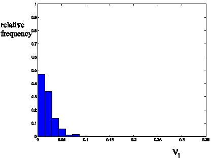
Figure 4: Histogram of n₁(t)

Figure 5: Histogram of n₃(t)

Figure 6: Histogram of n₆(t)

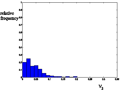
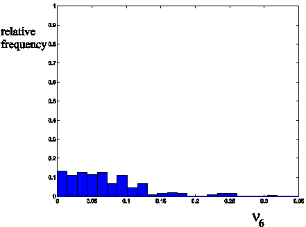
Table 3 shows the observations and the forecasted values. Note that in Table 3 in the first 46 observation times some values are evidenced in blue colour. These values are some of the most satisfactory forecasted values of a_t,m, m = 1,6 one month and six months in the future. We have computed the conditioned variance of the state variable z_t (formula (24)) corresponding to these forecasted values of the HFRI-Equity index. We observe that the conditioned variances relative to the forecasted values of the returns one month or six months in the future marked in blue are significantly smaller than the remaining ones. For example, while the mean value of the conditioned variances of the forecasted values of the returns of the HFRI-Equity index one month in the future is 1.27·10^-2 the value of the variances of the forecasted values marked in blue (in time order) are 7.4·10^-3, 4.4·10^-3, 6.1·10^-3, that is the conditioned variance of the blue forecasts is reduced of approximately a factor 0.5 with respect to its mean value. The same happens in the case of the forecasted values six months in the future where the mean value of the conditioned variance is 2.5·10^-2 and the conditioned variances of the forecasted values marked in blue (in time order) are 9.94·10^-3, 9.96·10^-3, 1.18·10^-2 and 1.23·10^-2. That is also in this last case the conditioned variances of the forecasted values marked in blue are reduced of approximately a factor 0.5 with respect to its mean value. This fact observed in the high quality forecasts contained in the first 46 observation times is confirmed when we look to the entire data time series. We have limited the study of the high quality forecasts to the first 46 observation times for simplicity. Similar results are obtained studying the forecasted values of the S&P 500 index.

This analysis shows that the conditioned variance allows us to assign a priori a degree of reliability to the corresponding forecasted value, that is: a small conditioned variance actually corresponds to a great degree of reliability of the corresponding forecasted value. This fact may be of great relevance in practical situations since using the conditioned variances we can evaluate a priori the quality of the forecasts of the HFRI-Equity index.

We conclude showing two digital movies concerning the forecasting problem.

The first movie shows the forecasted values one month , three months and six months in the future of the SP&500 index and of the HFRI Equity hedge fund index in comparison with the observed values, that is the point one, three, six months in the future is shown in the cartesian plane and compared with the corresponding observed points when the time t ranges in the observation period that goes from May 31, 1990 to December 31, 2006.

Click here to see the first movie

The second movie shows how the conditioned variances of the indices (see formulae (23), (24) ) can be used as a priori estimates of the quality of the forecasted values. In the movie we show the forecasted values of the variations of the log-return of the HFRI hedge fund index, the corresponding historical variations , i=1,2,…,N_tot ,m=1,3,6, and the corresponding conditioned variances. Note that when the conditioned variance of z_t is small the quality of the forecasted value is high.

Click here to see the second movie

5. References

[1] Y. Ait-Sahalia, R. Kimmel, Maximum likelihood estimation of stochastic volatility models, Journal of Financial Economics, 83 (2007), 413-452.

[2] D.S. Bates, Maximum likelihood estimation of latent affine processes, The Review of Financial Studies, 19 (2006), 909-965.

[3] F. Black, M. Scholes, The pricing of options and corporate liabilities, Journal of Political Economy, 81 (1973), 637-659.

[4] P. Capelli, F. Mariani, M.C. Recchioni, F. Spinelli, F.Zirilli, Determining a stable relationship between hedge fund index HFRI-Equity and S&P 500 behaviour, using filtering and maximum likelihood,Inverse Problems in Science and Engineering 18 (2010),83-109.

[5] L.Fatone, F. Mariani, M.C.Recchioni, F.Zirilli, Maximum likelihood estimation of the parameters of a system of stochastic differential equations that models the returns of the index of some classes of hedge funds, Journal of Inverse and Ill-Posed Problems, 15 (2007), 329-362, http://www.econ.univpm.it/recchioni/finance/w5.

[6] L. Fatone, F. Mariani, M.C. Recchioni, F.Zirilli, The calibration of the Heston stochastic volatility model using filtering and maximum likelihood methods, in Proceedings of Dynamic Systems and Applications, G.S.Ladde, N.G.Medhin, Chuang Peng, M.Sambandham Editors, Dynamic Publishers, Atlanta, USA, 5 (2008), 170-181, http://www.econ.univpm.it/recchioni/finance/w6.

[7] A. Harvey, R. Whaley, Market volatility prediction and the efficiency of the S&P 500 Index Option Market, Journal of Financial Economics, 31 (1992), 43-74.

[8] S.L. Heston, A closed-form solution for options with stochastic volatility with applications to bond and currency options, The Review of Financial Studies, 6 (1993), 327-343.

[9] F. Mariani, G. Pacelli, F. Zirilli, Maximum likelihood estimation of the Heston stochastic volatility model using asset and option prices: an application of nonlinear filtering theory, Optimization Letters, 2 (2008), 177-222, http://www.econ.univpm.it/pacelli/mariani/w1.

[10] P. Pillonel, L. Solanet, Predictability in hedge fund index returns and its application in fund of hedge funds style allocation, Master's Thesis in Banking and Finance at Université de Lausanne, Hautes Etudes Commerciales (HEC), 2006. (downloadable from the website:

http://www.hec.unil.ch/cms_mbf/master_thesis/0403.pdf).

TABLE 1: Historical data

i	date	variation HFRI Equity Hedge Index	variation S&P 500	HFRI Equity Hedge Index	S&P 500	HFRI Equity Hedge return	S&P 500 return
0	31/12/1989	--	--	---	---	0.00000	0.00000
1	31/01/1990	-3.34%	-6.88%	-3.340E-02	-6.880E-02	-0.03397	-0.07128
2	28/02/1990	2.85%	0.85%	2.850E-02	8.539E-03	-0.00587	-0.06278
3	31/03/1990	5.67%	2.43%	5.670E-02	2.426E-02	0.04928	-0.03881
4	30/04/1990	-0.87%	-2.69%	-8.700E-03	-2.689E-02	0.04054	-0.06607
5	31/05/1990	5.92%	9.20%	5.920E-02	9.199E-02	0.09806	0.02194
6	30/06/1990	2.52%	-0.89%	2.520E-02	-8.886E-03	0.12295	0.01301
7	31/07/1990	2.00%	-0.52%	2.000E-02	-5.223E-03	0.14275	0.00777
8	31/08/1990	-1.88%	-9.43%	-1.880E-02	-9.431E-02	0.12377	-0.09129
9	30/09/1990	1.65%	-5.12%	1.650E-02	-5.118E-02	0.14013	-0.14382
10	31/10/1990	0.77%	-0.67%	7.700E-03	-6.698E-03	0.14780	-0.15054
11	30/11/1990	-2.29%	5.99%	-2.290E-02	5.993E-02	0.12464	-0.09234
12	31/12/1990	1.02%	2.48%	1.020E-02	2.483E-02	0.13479	-0.06781
13	31/01/1991	4.90%	4.15%	4.900E-02	4.152E-02	0.18262	-0.02713
14	28/02/1991	5.20%	6.73%	5.200E-02	6.728E-02	0.23332	0.03798
15	31/03/1991	7.22%	2.22%	7.220E-02	2.220E-02	0.30303	0.05994
16	30/04/1991	0.47%	0.03%	4.700E-03	3.198E-04	0.30772	0.06026
17	31/05/1991	3.20%	3.86%	3.200E-02	3.860E-02	0.33922	0.09813
18	30/06/1991	0.59%	-4.79%	5.900E-03	-4.789E-02	0.34510	0.04906
19	31/07/1991	1.41%	4.49%	1.410E-02	4.486E-02	0.35910	0.09294
20	31/08/1991	2.17%	1.96%	2.170E-02	1.965E-02	0.38057	0.11240
21	30/09/1991	4.30%	-1.91%	4.300E-02	-1.914E-02	0.42267	0.09308
22	31/10/1991	1.16%	1.18%	1.160E-02	1.183E-02	0.43420	0.10484
23	30/11/1991	-1.08%	-4.39%	-1.080E-02	-4.390E-02	0.42335	0.05994
24	31/12/1991	5.02%	11.16%	5.020E-02	1.116E-01	0.47233	0.16574
25	31/01/1992	2.49%	-1.99%	2.490E-02	-1.990E-02	0.49692	0.14564
26	29/02/1992	2.90%	0.96%	2.900E-02	9.565E-03	0.52551	0.15516
27	31/03/1992	-0.28%	-2.18%	-2.800E-03	-2.183E-02	0.52270	0.13309
28	30/04/1992	0.27%	2.79%	2.700E-03	2.789E-02	0.52540	0.16060
29	31/05/1992	0.85%	0.10%	8.500E-03	9.640E-04	0.53386	0.16156
30	30/06/1992	-0.92%	-1.74%	-9.200E-03	-1.736E-02	0.52462	0.14405
31	31/07/1992	2.76%	3.94%	2.760E-02	3.940E-02	0.55185	0.18269
32	31/08/1992	-0.85%	-2.40%	-8.500E-03	-2.402E-02	0.54331	0.15838
33	30/09/1992	2.51%	0.91%	2.510E-02	9.106E-03	0.56810	0.16744
34	31/10/1992	2.03%	0.21%	2.030E-02	2.106E-03	0.58820	0.16955
35	30/11/1992	4.51%	3.03%	4.510E-02	3.026E-02	0.63231	0.19936
36	31/12/1992	3.38%	1.01%	3.380E-02	1.011E-02	0.66555	0.20942
37	31/01/1993	2.09%	0.70%	2.090E-02	7.046E-03	0.68624	0.21644
38	28/02/1993	-0.57%	1.05%	-5.700E-03	1.048E-02	0.68052	0.22687
39	31/03/1993	3.26%	1.87%	3.260E-02	1.870E-02	0.71260	0.24539
40	30/04/1993	1.30%	-2.54%	1.300E-02	-2.542E-02	0.72552	0.21964
41	31/05/1993	2.72%	2.27%	2.720E-02	2.272E-02	0.75235	0.24211
42	30/06/1993	3.01%	0.08%	3.010E-02	7.552E-04	0.78201	0.24287
43	31/07/1993	2.12%	-0.53%	2.120E-02	-5.327E-03	0.80299	0.23752
44	31/08/1993	3.84%	3.44%	3.840E-02	3.443E-02	0.84067	0.27137
45	30/09/1993	2.52%	-1.00%	2.520E-02	-9.988E-03	0.86556	0.26134
46	31/10/1993	3.11%	1.94%	3.110E-02	1.939E-02	0.89618	0.28054
47	30/11/1993	-1.93%	-1.29%	-1.930E-02	-1.291E-02	0.87669	0.26755
48	31/12/1993	3.59%	1.01%	3.590E-02	1.009E-02	0.91197	0.27759
49	31/01/1994	2.35%	3.25%	2.350E-02	3.250E-02	0.93519	0.30957
50	28/02/1994	-0.40%	-3.00%	-4.000E-03	-3.005E-02	0.93119	0.27906
51	31/03/1994	-2.08%	-4.57%	-2.080E-02	-4.575E-02	0.91017	0.23223
52	30/04/1994	-0.37%	1.15%	-3.700E-03	1.153E-02	0.90646	0.24369
53	31/05/1994	0.41%	1.24%	4.100E-03	1.242E-02	0.91055	0.25604
54	30/06/1994	-0.41%	-2.68%	-4.100E-03	-2.681E-02	0.90644	0.22886
55	31/07/1994	0.91%	3.15%	9.100E-03	3.149E-02	0.91550	0.25986
56	31/08/1994	1.27%	3.76%	1.270E-02	3.762E-02	0.92812	0.29679
57	30/09/1994	1.32%	-2.69%	1.320E-02	-2.690E-02	0.94123	0.26953
58	31/10/1994	0.40%	2.08%	4.000E-03	2.083E-02	0.94523	0.29014
59	30/11/1994	-1.48%	-3.95%	-1.480E-02	-3.950E-02	0.93032	0.24984
60	31/12/1994	0.74%	1.23%	7.400E-03	1.230E-02	0.93769	0.26207
61	31/01/1995	0.30%	2.43%	3.000E-03	2.428E-02	0.94068	0.28606
62	28/02/1995	1.68%	3.61%	1.680E-02	3.607E-02	0.95734	0.32149
63	31/03/1995	2.09%	2.73%	2.090E-02	2.733E-02	0.97803	0.34845
64	30/04/1995	2.64%	2.80%	2.640E-02	2.796E-02	1.00409	0.37603
65	31/05/1995	1.22%	3.63%	1.220E-02	3.631E-02	1.01621	0.41170
66	30/06/1995	4.73%	2.13%	4.730E-02	2.128E-02	1.06243	0.43275
67	31/07/1995	4.46%	3.18%	4.460E-02	3.178E-02	1.10606	0.46404
68	31/08/1995	2.93%	-0.03%	2.930E-02	-3.203E-04	1.13494	0.46372
69	30/09/1995	2.90%	4.01%	2.900E-02	4.010E-02	1.16353	0.50303
70	31/10/1995	-1.44%	-0.50%	-1.440E-02	-4.979E-03	1.14902	0.49804
71	30/11/1995	3.43%	4.10%	3.430E-02	4.105E-02	1.18275	0.53827
72	31/12/1995	2.56%	1.74%	2.560E-02	1.744E-02	1.20803	0.55556
73	31/01/1996	1.06%	3.26%	1.060E-02	3.262E-02	1.21857	0.58766
74	29/02/1996	2.82%	0.69%	2.820E-02	6.934E-03	1.24638	0.59457
75	31/03/1996	1.90%	0.79%	1.900E-02	7.917E-03	1.26520	0.60246
76	30/04/1996	5.34%	1.34%	5.340E-02	1.343E-02	1.31723	0.61580
77	31/05/1996	3.70%	2.29%	3.700E-02	2.285E-02	1.35356	0.63839
78	30/06/1996	-0.73%	0.23%	-7.300E-03	2.257E-03	1.34623	0.64065
79	31/07/1996	-2.87%	-4.57%	-2.870E-02	-4.575E-02	1.31711	0.59382
80	31/08/1996	2.63%	1.88%	2.630E-02	1.881E-02	1.34307	0.61245
81	30/09/1996	2.18%	5.42%	2.180E-02	5.417E-02	1.36464	0.66521
82	31/10/1996	1.56%	2.61%	1.560E-02	2.613E-02	1.38012	0.69100
83	30/11/1996	1.66%	7.34%	1.660E-02	7.338E-02	1.39658	0.76181
84	31/12/1996	0.83%	-2.15%	8.300E-03	-2.151E-02	1.40485	0.74007
85	31/01/1997	2.78%	6.13%	2.780E-02	6.132E-02	1.43227	0.79958
86	28/02/1997	-0.24%	0.59%	-2.400E-03	5.928E-03	1.42986	0.80549
87	31/03/1997	-0.73%	-4.26%	-7.300E-03	-4.261E-02	1.42254	0.76195
88	30/04/1997	-0.27%	5.84%	-2.700E-03	5.841E-02	1.41983	0.81871
89	31/05/1997	5.04%	5.86%	5.040E-02	5.858E-02	1.46900	0.87564
90	30/06/1997	1.97%	4.35%	1.970E-02	4.345E-02	1.48851	0.91818
91	31/07/1997	5.05%	7.81%	5.050E-02	7.812E-02	1.53778	0.99339
92	31/08/1997	1.35%	-5.74%	1.350E-02	-5.745E-02	1.55119	0.93423
93	30/09/1997	5.69%	5.32%	5.690E-02	5.315E-02	1.60653	0.98601
94	31/10/1997	0.39%	-3.45%	3.900E-03	-3.448E-02	1.61042	0.95093
95	30/11/1997	-0.93%	4.46%	-9.300E-03	4.459E-02	1.60108	0.99455
96	31/12/1997	1.42%	1.57%	1.420E-02	1.573E-02	1.61518	1.01016
97	31/01/1998	-0.16%	1.02%	-1.600E-03	1.015E-02	1.61358	1.02026
98	28/02/1998	4.09%	7.04%	4.090E-02	7.045E-02	1.65366	1.08834
99	31/03/1998	4.54%	4.99%	4.540E-02	4.995E-02	1.69806	1.13708
100	30/04/1998	1.39%	0.91%	1.390E-02	9.076E-03	1.71187	1.14611
101	31/05/1998	-1.27%	-1.88%	-1.270E-02	-1.883E-02	1.69908	1.12710
102	30/06/1998	0.50%	3.94%	5.000E-03	3.944E-02	1.70407	1.16579
103	31/07/1998	-0.67%	-1.16%	-6.700E-03	-1.162E-02	1.69735	1.15410
104	31/08/1998	-7.65%	-14.58%	-7.650E-02	-1.458E-01	1.61777	0.99651
105	30/09/1998	3.16%	6.24%	3.160E-02	6.240E-02	1.64888	1.05704
106	31/10/1998	2.47%	8.03%	2.470E-02	8.029E-02	1.67328	1.13427
107	30/11/1998	3.84%	5.91%	3.840E-02	5.913E-02	1.71096	1.19172
108	31/12/1998	5.39%	5.64%	5.390E-02	5.638E-02	1.76345	1.24656
109	31/01/1999	4.98%	4.10%	4.980E-02	4.101E-02	1.81205	1.28675
110	28/02/1999	-2.41%	-3.23%	-2.410E-02	-3.228E-02	1.78766	1.25394
111	31/03/1999	4.05%	3.88%	4.050E-02	3.879E-02	1.82736	1.29200
112	30/04/1999	5.25%	3.79%	5.250E-02	3.794E-02	1.87853	1.32924
113	31/05/1999	1.22%	-2.50%	1.220E-02	-2.497E-02	1.89066	1.30395
114	30/06/1999	3.80%	5.44%	3.800E-02	5.444E-02	1.92795	1.35696
115	31/07/1999	0.61%	-3.20%	6.100E-03	-3.205E-02	1.93403	1.32438
116	31/08/1999	0.04%	-0.63%	4.000E-04	-6.254E-03	1.93443	1.31811
117	30/09/1999	0.35%	-2.86%	3.500E-03	-2.855E-02	1.93793	1.28915
118	31/10/1999	2.33%	6.25%	2.330E-02	6.254E-02	1.96096	1.34981
119	30/11/1999	6.76%	1.91%	6.760E-02	1.906E-02	2.02637	1.36869
120	31/12/1999	10.88%	5.78%	1.088E-01	5.784E-02	2.12965	1.42492
121	31/01/2000	0.25%	-5.09%	2.500E-03	-5.090E-02	2.13215	1.37268
122	29/02/2000	10.00%	-2.01%	1.000E-01	-2.011E-02	2.22746	1.35236
123	31/03/2000	1.73%	9.67%	1.730E-02	9.672E-02	2.24461	1.44469
124	30/04/2000	-4.19%	-3.08%	-4.190E-02	-3.080E-02	2.20181	1.41340
125	31/05/2000	-2.44%	-2.19%	-2.440E-02	-2.191E-02	2.17710	1.39125
126	30/06/2000	4.85%	2.39%	4.850E-02	2.393E-02	2.22446	1.41490
127	31/07/2000	-1.58%	-1.63%	-1.580E-02	-1.634E-02	2.20854	1.39842
128	31/08/2000	5.35%	6.07%	5.350E-02	6.070E-02	2.26066	1.45735
129	30/09/2000	-1.08%	-5.35%	-1.080E-02	-5.348E-02	2.24980	1.40239
130	31/10/2000	-2.01%	-0.49%	-2.010E-02	-4.949E-03	2.22949	1.39743
131	30/11/2000	-4.30%	-8.01%	-4.300E-02	-8.007E-02	2.18554	1.31397
132	31/12/2000	3.16%	0.41%	3.160E-02	4.053E-03	2.21665	1.31801
133	31/01/2001	2.88%	3.46%	2.880E-02	3.464E-02	2.24504	1.35207
134	28/02/2001	-2.56%	-9.23%	-2.560E-02	-9.229E-02	2.21911	1.25524
135	31/03/2001	-2.30%	-6.42%	-2.300E-02	-6.420E-02	2.19584	1.18888
136	30/04/2001	2.27%	7.68%	2.270E-02	7.681E-02	2.21829	1.26289
137	31/05/2001	0.90%	0.51%	9.000E-03	5.090E-03	2.22725	1.26796
138	30/06/2001	-0.32%	-2.50%	-3.200E-03	-2.500E-02	2.22404	1.24264
139	31/07/2001	-1.06%	-1.08%	-1.060E-02	-1.077E-02	2.21339	1.23182
140	31/08/2001	-1.22%	-6.41%	-1.220E-02	-6.411E-02	2.20111	1.16556
141	30/09/2001	-3.73%	-8.17%	-3.730E-02	-8.172E-02	2.16310	1.08031
142	31/10/2001	1.85%	1.81%	1.850E-02	1.810E-02	2.18143	1.09824
143	30/11/2001	1.97%	7.52%	1.970E-02	7.518E-02	2.20094	1.17073
144	31/12/2001	1.99%	0.76%	1.990E-02	7.574E-03	2.22064	1.17828
145	31/01/2002	0.22%	-1.56%	2.200E-03	-1.557E-02	2.22284	1.16258
146	28/02/2002	-0.89%	-2.08%	-8.900E-03	-2.077E-02	2.21390	1.14160
147	31/03/2002	2.03%	3.67%	2.030E-02	3.674E-02	2.23400	1.17768
148	30/04/2002	0.17%	-6.14%	1.700E-03	-6.142E-02	2.23570	1.11429
149	31/05/2002	0.00%	-0.91%	0.000E+00	-9.081E-03	2.23570	1.10517
150	30/06/2002	-2.63%	-7.25%	-2.630E-02	-7.246E-02	2.20904	1.02995
151	31/07/2002	-3.93%	-7.90%	-3.930E-02	-7.900E-02	2.16895	0.94765
152	31/08/2002	0.28%	0.49%	2.800E-03	4.881E-03	2.17175	0.95252
153	30/09/2002	-1.96%	-11.00%	-1.960E-02	-1.100E-01	2.15195	0.83599
154	31/10/2002	0.56%	8.64%	5.600E-03	8.645E-02	2.15754	0.91890
155	30/11/2002	2.67%	5.71%	2.670E-02	5.707E-02	2.18389	0.97440
156	31/12/2002	-1.14%	-6.03%	-1.140E-02	-6.033E-02	2.17242	0.91218
157	31/01/2003	-0.01%	-2.74%	-1.000E-04	-2.741E-02	2.17232	0.88439
158	28/02/2003	-0.78%	-1.70%	-7.800E-03	-1.700E-02	2.16449	0.86724
159	31/03/2003	-0.07%	0.84%	-7.000E-04	8.358E-03	2.16379	0.87556
160	30/04/2003	2.43%	8.10%	2.430E-02	8.104E-02	2.18780	0.95349
161	31/05/2003	4.08%	5.09%	4.080E-02	5.090E-02	2.22779	1.00313
162	30/06/2003	1.52%	1.13%	1.520E-02	1.132E-02	2.24287	1.01439
163	31/07/2003	2.41%	1.62%	2.410E-02	1.622E-02	2.26669	1.03048
164	31/08/2003	2.38%	1.79%	2.380E-02	1.787E-02	2.29021	1.04819
165	30/09/2003	0.78%	-1.19%	7.800E-03	-1.194E-02	2.29798	1.03618
166	31/10/2003	3.12%	5.50%	3.120E-02	5.496E-02	2.32870	1.08968
167	30/11/2003	1.14%	0.71%	1.140E-02	7.129E-03	2.34004	1.09679
168	31/12/2003	1.93%	5.08%	1.930E-02	5.077E-02	2.35915	1.14631
169	31/01/2004	1.95%	1.73%	1.950E-02	1.728E-02	2.37847	1.16344
170	29/02/2004	1.11%	1.22%	1.110E-02	1.221E-02	2.38951	1.17558
171	31/03/2004	0.36%	-1.64%	3.600E-03	-1.636E-02	2.39310	1.15908
172	30/04/2004	-2.08%	-1.68%	-2.080E-02	-1.679E-02	2.37208	1.14215
173	31/05/2004	-0.19%	1.21%	-1.900E-03	1.208E-02	2.37018	1.15416
174	30/06/2004	1.07%	1.80%	1.070E-02	1.799E-02	2.38082	1.17199
175	31/07/2004	-1.88%	-3.43%	-1.880E-02	-3.429E-02	2.36184	1.13710
176	31/08/2004	-0.37%	0.23%	-3.700E-03	2.287E-03	2.35814	1.13938
177	30/09/2004	1.99%	0.94%	1.990E-02	9.364E-03	2.37784	1.14870
178	31/10/2004	0.48%	1.40%	4.800E-03	1.401E-02	2.38263	1.16261
179	30/11/2004	3.37%	3.86%	3.370E-02	3.859E-02	2.41577	1.20048
180	31/12/2004	1.76%	3.25%	1.760E-02	3.246E-02	2.43322	1.23242
181	31/01/2005	-0.58%	-2.53%	-5.800E-03	-2.529E-02	2.42740	1.20681
182	28/02/2005	2.13%	1.89%	2.130E-02	1.890E-02	2.44848	1.22553
183	31/03/2005	-1.05%	-1.91%	-1.050E-02	-1.912E-02	2.43792	1.20623
184	30/04/2005	-2.23%	-2.01%	-2.230E-02	-2.011E-02	2.41537	1.18591
185	31/05/2005	1.55%	3.00%	1.550E-02	2.995E-02	2.43075	1.21542
186	30/06/2005	1.96%	-0.01%	1.960E-02	-1.427E-04	2.45016	1.21528
187	31/07/2005	2.95%	3.60%	2.950E-02	3.597E-02	2.47924	1.25062
188	31/08/2005	0.74%	-1.12%	7.400E-03	-1.122E-02	2.48661	1.23933
189	30/09/2005	2.25%	0.69%	2.250E-02	6.949E-03	2.50886	1.24626
190	31/10/2005	-1.87%	-1.77%	-1.870E-02	-1.774E-02	2.48998	1.22836
191	30/11/2005	2.14%	3.52%	2.140E-02	3.519E-02	2.51116	1.26294
192	31/12/2005	2.32%	-0.10%	2.320E-02	-9.524E-04	2.53409	1.26199
193	31/01/2006	3.95%	2.55%	3.950E-02	2.547E-02	2.57283	1.28714
194	28/02/2006	0.02%	0.05%	2.000E-04	4.531E-04	2.57303	1.28759
195	31/03/2006	2.55%	1.11%	2.550E-02	1.106E-02	2.59821	1.29859
196	30/04/2006	1.76%	1.22%	1.760E-02	1.219E-02	2.61566	1.31071
197	31/05/2006	-2.32%	-3.09%	-2.320E-02	-3.092E-02	2.59219	1.27930
198	30/06/2006	-0.54%	0.01%	-5.400E-03	8.661E-05	2.58677	1.27939
199	31/07/2006	-0.54%	0.51%	-5.400E-03	5.086E-03	2.58136	1.28446
200	31/08/2006	1.03%	2.13%	1.030E-02	2.127E-02	2.59160	1.30551
201	30/09/2006	0.16%	2.46%	1.600E-03	2.457E-02	2.59320	1.32978
202	31/10/2006	1.86%	3.15%	1.860E-02	3.151E-02	2.61163	1.36081
203	30/11/2006	2.00%	1.65%	2.000E-02	1.647E-02	2.63143	1.37714
204	31/12/2006	1.35%	1.26%	1.350E-02	1.262E-02	2.64484	1.38968
205	31/01/2007	1.16%	1.41%	1.160E-02	1.406E-02	2.65638	1.40364
206	28/02/2007	0.63%	-2.18%	6.300E-03	-2.185E-02	2.66266	1.38155
207	31/03/2007	1.02%	1.00%	1.020E-02	9.980E-03	2.67281	1.39148
208	30/04/2007	1.95%	4.33%	1.950E-02	4.329E-02	2.69212	1.43386
209	31/05/2007	2.29%	3.25%	2.290E-02	3.255E-02	2.71476	1.46589
210	30/06/2007	1.09%	-1.78%	1.090E-02	-1.782E-02	2.72560	1.44791

TABLE 3: Forecasted values of the log-returns

i	date	one month variation (in per cent) of the S&P 500 index	one month variation (in per cent) of the HFRI Equity hedge fund index	observed one month return	forecasted one month return	observed six months return	forecasted six months return
1	31/01/1990	-6.88%	-3.34%
2	28/02/1990	0.85%	2.85%
3	31/03/1990	2.43%	5.67%
4	30/04/1990	-2.69%	-0.87%
5	31/05/1990	9.20%	5.92%
6	30/06/1990	-0.89%	2.52%	2.52E-02	6.55E-03
7	31/07/1990	-0.52%	2.00%	2.00E-02	1.18E-02
8	31/08/1990	-9.43%	-1.88%	-1.88E-02	1.10E-02
9	30/09/1990	-5.12%	1.65%	1.65E-02	4.48E-03
10	31/10/1990	-0.67%	0.77%	7.70E-03	6.66E-03
11	30/11/1990	5.99%	-2.29%	-2.29E-02	2.33E-03	2.694E-02	3.993E-02
12	31/12/1990	2.48%	1.02%	1.02E-02	1.63E-03	1.191E-02	7.308E-02
13	31/01/1991	4.15%	4.90%	4.90E-02	-2.97E-03	4.068E-02	6.786E-02
14	28/02/1991	6.73%	5.20%	5.20E-02	3.42E-03	1.158E-01	2.717E-02
15	31/03/1991	2.22%	7.22%	7.22E-02	6.43E-03	1.769E-01	4.062E-02
16	30/04/1991	0.03%	0.47%	4.70E-03	2.00E-02	1.734E-01	1.409E-02
17	31/05/1991	3.86%	3.20%	3.20E-02	1.53E-02	2.393E-01	9.814E-03
18	30/06/1991	-4.79%	0.59%	5.90E-03	1.64E-02	2.341E-01	-1.766E-02
19	31/07/1991	4.49%	1.41%	1.41E-02	2.28E-02	1.930E-01	2.071E-02
20	31/08/1991	1.96%	2.17%	2.17E-02	5.36E-03	1.586E-01	3.921E-02
21	30/09/1991	-1.91%	4.30%	4.30E-02	6.54E-03	1.271E-01	1.262E-01
22	31/10/1991	1.18%	1.16%	1.16E-02	1.34E-02	1.348E-01	9.517E-02
23	30/11/1991	-4.39%	-1.08%	-1.08E-02	1.18E-02	8.777E-02	1.026E-01
24	31/12/1991	11.16%	5.02%	5.02E-02	1.00E-02	1.357E-01	1.445E-01
25	31/01/1992	-1.99%	2.49%	2.49E-02	1.48E-02	1.478E-01	3.261E-02
26	29/02/1992	0.96%	2.90%	2.90E-02	1.72E-02	1.560E-01	3.990E-02
27	31/03/1992	-2.18%	-0.28%	-2.80E-03	1.35E-02	1.052E-01	8.335E-02
28	30/04/1992	2.79%	0.27%	2.70E-03	1.06E-02	9.548E-02	7.318E-02
29	31/05/1992	0.10%	0.85%	8.50E-03	1.59E-02	1.169E-01	6.176E-02
30	30/06/1992	-1.74%	-0.92%	-9.20E-03	8.66E-03	5.369E-02	9.231E-02
31	31/07/1992	3.94%	2.76%	2.76E-02	4.94E-03	5.646E-02	1.079E-01
32	31/08/1992	-2.40%	-0.85%	-8.50E-03	4.88E-03	1.796E-02	8.346E-02
33	30/09/1992	0.91%	2.51%	2.51E-02	4.50E-03	4.644E-02	6.531E-02
34	31/10/1992	0.21%	2.03%	2.03E-02	4.80E-03	6.481E-02	9.928E-02
35	30/11/1992	3.03%	4.51%	4.51E-02	4.37E-03	1.035E-01	5.308E-02
36	31/12/1992	1.01%	3.38%	3.38E-02	1.22E-02	1.513E-01	3.001E-02
37	31/01/1993	0.70%	2.09%	2.09E-02	1.30E-02	1.438E-01	2.966E-02
38	28/02/1993	1.05%	-0.57%	-5.70E-03	1.90E-02	1.471E-01	2.731E-02
39	31/03/1993	1.87%	3.26%	3.26E-02	1.22E-02	1.555E-01	2.913E-02
40	30/04/1993	-2.54%	1.30%	1.30E-02	1.62E-02	1.472E-01	2.654E-02
41	31/05/1993	2.27%	2.72%	2.72E-02	1.18E-02	1.275E-01	7.539E-02
42	30/06/1993	0.08%	3.01%	3.01E-02	1.04E-02	1.235E-01	8.066E-02
43	31/07/1993	-0.53%	2.12%	2.12E-02	1.36E-02	1.238E-01	1.195E-01
44	31/08/1993	3.44%	3.84%	3.84E-02	1.54E-02	1.737E-01	7.566E-02
45	30/09/1993	-1.00%	2.52%	2.52E-02	1.75E-02	1.653E-01	1.015E-01
46	31/10/1993	1.94%	3.11%	3.11E-02	1.84E-02	1.861E-01	7.300E-02
47	30/11/1993	-1.29%	-1.93%	-1.93E-02	1.91E-02	1.324E-01	6.430E-02
48	31/12/1993	1.01%	3.59%	3.59E-02	1.23E-02	1.388E-01	8.470E-02
49	31/01/1994	3.25%	2.35%	2.35E-02	1.28E-02	1.413E-01	9.576E-02
50	28/02/1994	-3.00%	-0.40%	-4.00E-03	1.20E-02	9.474E-02	1.095E-01
51	31/03/1994	-4.57%	-2.08%	-2.08E-02	7.95E-03	4.562E-02	1.158E-01
52	30/04/1994	1.15%	-0.37%	-3.70E-03	4.35E-03	1.033E-02	1.202E-01
53	31/05/1994	1.24%	0.41%	4.10E-03	3.93E-03	3.444E-02	7.632E-02
54	30/06/1994	-2.68%	-0.41%	-4.10E-03	-1.39E-03	-5.508E-03	7.920E-02
55	31/07/1994	3.15%	0.91%	9.10E-03	-5.35E-03	-1.950E-02	7.448E-02
56	31/08/1994	3.76%	1.27%	1.27E-02	-3.47E-03	-3.059E-03	4.868E-02
57	30/09/1994	-2.69%	1.32%	1.32E-02	4.48E-03	3.156E-02	2.639E-02
58	31/10/1994	2.08%	0.40%	4.00E-03	4.21E-03	3.953E-02	2.381E-02
59	30/11/1994	-3.95%	-1.48%	-1.48E-02	2.82E-03	1.996E-02	-8.331E-03
60	31/12/1994	1.23%	0.74%	7.40E-03	2.45E-03	3.174E-02	-3.169E-02
61	31/01/1995	2.43%	0.30%	3.00E-03	2.54E-03	2.550E-02	-2.064E-02
62	28/02/1995	3.61%	1.68%	1.68E-02	4.04E-03	2.965E-02	2.718E-02
63	31/03/1995	2.73%	2.09%	2.09E-02	2.54E-03	3.748E-02	2.555E-02
64	30/04/1995	2.80%	2.64%	2.64E-02	4.70E-03	6.063E-02	1.705E-02
65	31/05/1995	3.63%	1.22%	1.22E-02	9.33E-03	8.969E-02	1.477E-02
66	30/06/1995	2.13%	4.73%	4.73E-02	9.14E-03	1.329E-01	1.536E-02
67	31/07/1995	3.18%	4.46%	4.46E-02	1.59E-02	1.798E-01	2.448E-02
68	31/08/1995	-0.03%	2.93%	2.93E-02	1.89E-02	1.943E-01	1.535E-02
69	30/09/1995	4.01%	2.90%	2.90E-02	2.14E-02	2.038E-01	2.852E-02
70	31/10/1995	-0.50%	-1.44%	-1.44E-02	1.92E-02	1.560E-01	5.730E-02
71	30/11/1995	4.10%	3.43%	3.43E-02	1.72E-02	1.812E-01	5.608E-02
72	31/12/1995	1.74%	2.56%	2.56E-02	1.57E-02	1.567E-01	9.919E-02
73	31/01/1996	3.26%	1.06%	1.06E-02	1.32E-02	1.191E-01	1.188E-01
74	29/02/1996	0.69%	2.82%	2.82E-02	1.06E-02	1.179E-01	1.352E-01
75	31/03/1996	0.79%	1.90%	1.90E-02	1.07E-02	1.070E-01	1.211E-01
76	30/04/1996	1.34%	5.34%	5.34E-02	1.56E-02	1.832E-01	1.078E-01
77	31/05/1996	2.29%	3.70%	3.70E-02	1.85E-02	1.863E-01	9.766E-02
78	30/06/1996	0.23%	-0.73%	-7.30E-03	2.00E-02	1.482E-01	8.200E-02
79	31/07/1996	-4.57%	-2.87%	-2.87E-02	1.66E-02	1.036E-01	6.507E-02
80	31/08/1996	1.88%	2.63%	2.63E-02	8.76E-03	1.015E-01	6.613E-02
81	30/09/1996	5.42%	2.18%	2.18E-02	9.14E-03	1.045E-01	9.762E-02
82	31/10/1996	2.61%	1.56%	1.56E-02	5.59E-03	6.491E-02	1.163E-01
83	30/11/1996	7.34%	1.66%	1.66E-02	4.54E-03	4.396E-02	1.263E-01
84	31/12/1996	-2.15%	0.83%	8.30E-03	6.47E-03	6.037E-02	1.038E-01
85	31/01/1997	6.13%	2.78%	2.78E-02	1.19E-02	1.220E-01	5.374E-02
86	28/02/1997	0.59%	-0.24%	-2.40E-03	1.14E-02	9.067E-02	5.610E-02
87	31/03/1997	-4.26%	-0.73%	-7.30E-03	8.02E-03	5.961E-02	3.398E-02
88	30/04/1997	5.84%	-0.27%	-2.70E-03	4.68E-03	4.052E-02	2.753E-02
89	31/05/1997	5.86%	5.04%	5.04E-02	4.58E-03	7.511E-02	3.942E-02
90	30/06/1997	4.35%	1.97%	1.97E-02	7.34E-03	8.727E-02	7.370E-02
91	31/07/1997	7.81%	5.05%	5.05E-02	6.88E-03	1.113E-01	7.040E-02
92	31/08/1997	-5.74%	1.35%	1.35E-02	1.40E-02	1.290E-01	4.910E-02
93	30/09/1997	5.32%	5.69%	5.69E-02	1.86E-02	2.020E-01	2.842E-02
94	31/10/1997	-3.45%	0.39%	3.90E-03	2.43E-02	2.100E-01	2.779E-02
95	30/11/1997	4.46%	-0.93%	-9.30E-03	1.84E-02	1.412E-01	4.482E-02
96	31/12/1997	1.57%	1.42%	1.42E-02	9.80E-03	1.350E-01	4.199E-02
97	31/01/1998	1.02%	-0.16%	-1.60E-03	6.82E-03	7.874E-02	8.665E-02
98	28/02/1998	7.04%	4.09%	4.09E-02	6.72E-03	1.079E-01	1.172E-01
99	31/03/1998	4.99%	4.54%	4.54E-02	4.78E-03	9.585E-02	1.551E-01
100	30/04/1998	0.91%	1.39%	1.39E-02	9.83E-03	1.068E-01	1.154E-01
101	31/05/1998	-1.88%	-1.27%	-1.27E-02	1.26E-02	1.030E-01	6.026E-02
102	30/06/1998	3.94%	0.50%	5.00E-03	1.06E-02	9.297E-02	4.161E-02
103	31/07/1998	-1.16%	-0.67%	-6.70E-03	1.10E-02	8.738E-02	4.100E-02
104	31/08/1998	-14.58%	-7.65%	-7.65E-02	4.39E-03	-3.526E-02	2.904E-02
105	30/09/1998	6.24%	3.16%	3.16E-02	-8.70E-03	-4.800E-02	6.042E-02
106	31/10/1998	8.03%	2.47%	2.47E-02	-9.49E-03	-3.785E-02	7.819E-02
107	30/11/1998	5.91%	3.84%	3.84E-02	-4.50E-03	1.194E-02	6.498E-02
108	31/12/1998	5.64%	5.39%	5.39E-02	4.29E-03	6.118E-02	6.790E-02
109	31/01/1999	4.10%	4.98%	4.98E-02	5.03E-03	1.215E-01	2.662E-02
110	28/02/1999	-3.23%	-2.41%	-2.41E-02	2.63E-02	1.852E-01	-5.108E-02
111	31/03/1999	3.88%	4.05%	4.05E-02	1.56E-02	1.954E-01	-5.558E-02
112	30/04/1999	3.79%	5.25%	5.25E-02	1.37E-02	2.278E-01	-2.667E-02
113	31/05/1999	-2.50%	1.22%	1.22E-02	1.95E-02	1.969E-01	2.602E-02
114	30/06/1999	5.44%	3.80%	3.80E-02	2.72E-02	1.788E-01	3.055E-02
115	31/07/1999	-3.20%	0.61%	6.10E-03	1.60E-02	1.297E-01	1.686E-01
116	31/08/1999	-0.63%	0.04%	4.00E-04	1.99E-02	1.581E-01	9.733E-02
117	30/09/1999	-2.86%	0.35%	3.50E-03	1.55E-02	1.169E-01	8.488E-02
118	31/10/1999	6.25%	2.33%	2.33E-02	7.13E-03	8.592E-02	1.228E-01
119	30/11/1999	1.91%	6.76%	6.76E-02	7.55E-03	1.454E-01	1.746E-01
120	31/12/1999	5.78%	10.88%	1.09E-01	1.56E-02	2.235E-01	9.959E-02
121	31/01/2000	-5.09%	0.25%	2.50E-03	2.53E-02	2.191E-01	1.253E-01
122	29/02/2000	-2.01%	10.00%	1.00E-01	2.19E-02	3.405E-01	9.659E-02
123	31/03/2000	9.67%	1.73%	1.73E-02	3.03E-02	3.589E-01	4.357E-02
124	30/04/2000	-3.08%	-4.19%	-4.19E-02	3.70E-02	2.723E-01	4.614E-02
125	31/05/2000	-2.19%	-2.44%	-2.44E-02	2.26E-02	1.627E-01	9.711E-02
126	30/06/2000	2.39%	4.85%	4.85E-02	5.99E-03	9.945E-02	1.614E-01
127	31/07/2000	-1.63%	-1.58%	-1.58E-02	1.24E-02	7.938E-02	1.391E-01
128	31/08/2000	6.07%	5.35%	5.35E-02	-3.54E-03	3.376E-02	1.964E-01
129	30/09/2000	-5.35%	-1.08%	-1.08E-02	4.74E-03	5.201E-03	2.432E-01
130	31/10/2000	-0.49%	-2.01%	-2.01E-02	6.00E-03	2.807E-02	1.436E-01
131	30/11/2000	-8.01%	-4.30%	-4.30E-02	5.76E-03	8.473E-03	3.648E-02
132	31/12/2000	0.41%	3.16%	3.16E-02	-7.03E-03	-7.782E-03	7.690E-02
133	31/01/2001	3.46%	2.88%	2.88E-02	4.59E-03	3.718E-02	-2.107E-02
134	28/02/2001	-9.23%	-2.56%	-2.56E-02	-3.07E-03	-4.069E-02	2.877E-02
135	31/03/2001	-6.42%	-2.30%	-2.30E-02	-6.21E-03	-5.252E-02	3.656E-02
136	30/04/2001	7.68%	2.27%	2.27E-02	-6.29E-03	-1.114E-02	3.509E-02
137	31/05/2001	0.51%	0.90%	9.00E-03	4.25E-03	4.259E-02	-4.145E-02
138	30/06/2001	-2.50%	-0.32%	-3.20E-03	4.23E-03	7.419E-03	2.786E-02
139	31/07/2001	-1.08%	-1.06%	-1.06E-02	-4.85E-03	-3.116E-02	-1.829E-02
140	31/08/2001	-6.41%	-1.22%	-1.22E-02	-2.40E-03	-1.784E-02	-3.670E-02
141	30/09/2001	-8.17%	-3.73%	-3.73E-02	3.70E-03	-3.221E-02	-3.718E-02
142	31/10/2001	1.81%	1.85%	1.85E-02	-7.58E-03	-3.619E-02	2.577E-02
143	30/11/2001	7.52%	1.97%	1.97E-02	-7.25E-03	-2.597E-02	2.566E-02
144	31/12/2001	0.76%	1.99%	1.99E-02	-3.83E-03	-3.395E-03	-2.873E-02
145	31/01/2002	-1.56%	0.22%	2.20E-03	3.94E-03	9.498E-03	-1.429E-02
146	28/02/2002	-2.08%	-0.89%	-8.90E-03	3.89E-03	1.287E-02	2.241E-02
147	31/03/2002	3.67%	2.03%	2.03E-02	5.07E-03	7.347E-02	-4.462E-02
148	30/04/2002	-6.14%	0.17%	1.70E-03	5.29E-03	5.577E-02	-4.273E-02
149	31/05/2002	-0.91%	0.00%	-2.13E-18	3.90E-03	3.537E-02	-2.273E-02
150	30/06/2002	-7.25%	-2.63%	-2.63E-02	3.47E-03	-1.153E-02	2.390E-02
151	31/07/2002	-7.90%	-3.93%	-3.93E-02	-2.57E-03	-5.246E-02	2.360E-02
152	31/08/2002	0.49%	0.28%	2.80E-03	-7.13E-03	-4.128E-02	3.082E-02
153	30/09/2002	-11.00%	-1.96%	-1.96E-02	-9.70E-03	-7.877E-02	3.213E-02
154	31/10/2002	8.64%	0.56%	5.60E-03	-1.28E-02	-7.518E-02	2.366E-02
155	30/11/2002	5.71%	2.67%	2.67E-02	-1.10E-02	-5.049E-02	2.099E-02
156	31/12/2002	-6.03%	-1.14%	-1.14E-02	-5.42E-03	-3.596E-02	-1.532E-02
157	31/01/2003	-2.74%	-0.01%	-1.00E-04	3.66E-03	3.376E-03	-4.204E-02
158	28/02/2003	-1.70%	-0.78%	-7.80E-03	3.44E-03	-7.230E-03	-5.680E-02
159	31/03/2003	0.84%	-0.07%	-7.00E-04	3.95E-03	1.191E-02	-7.432E-02
160	30/04/2003	8.10%	2.43%	2.43E-02	3.83E-03	3.073E-02	-6.428E-02
161	31/05/2003	5.09%	4.08%	4.08E-02	3.65E-03	4.488E-02	-3.206E-02
162	30/06/2003	1.13%	1.52%	1.52E-02	5.84E-03	7.300E-02	2.218E-02
163	31/07/2003	1.62%	2.41%	2.41E-02	7.43E-03	9.896E-02	2.083E-02
164	31/08/2003	1.79%	2.38%	2.38E-02	1.29E-02	1.340E-01	2.393E-02
165	30/09/2003	-1.19%	0.78%	7.80E-03	1.81E-02	1.436E-01	2.322E-02
166	31/10/2003	5.50%	3.12%	3.12E-02	1.27E-02	1.513E-01	2.211E-02
167	30/11/2003	0.71%	1.14%	1.14E-02	1.06E-02	1.188E-01	3.554E-02
168	31/12/2003	5.08%	1.93%	1.93E-02	1.17E-02	1.233E-01	4.541E-02
169	31/01/2004	1.73%	1.95%	1.95E-02	1.13E-02	1.183E-01	8.010E-02
170	29/02/2004	1.22%	1.11%	1.11E-02	1.26E-02	1.044E-01	1.139E-01
171	31/03/2004	-1.64%	0.36%	3.60E-03	1.10E-02	9.979E-02	7.886E-02
172	30/04/2004	-1.68%	-2.08%	-2.08E-02	7.38E-03	4.433E-02	6.536E-02
173	31/05/2004	1.21%	-0.19%	-1.90E-03	3.97E-03	3.060E-02	7.245E-02
174	30/06/2004	1.80%	1.07%	1.07E-02	4.15E-03	2.190E-02	7.000E-02
175	31/07/2004	-3.43%	-1.88%	-1.88E-02	4.50E-03	-1.649E-02	7.810E-02
176	31/08/2004	0.23%	-0.37%	-3.70E-03	-5.65E-03	-3.088E-02	6.801E-02
177	30/09/2004	0.94%	1.99%	1.99E-02	-6.59E-03	-1.514E-02	4.512E-02
178	31/10/2004	1.40%	0.48%	4.80E-03	4.11E-03	1.060E-02	2.406E-02
179	30/11/2004	3.86%	3.37%	3.37E-02	4.19E-03	4.665E-02	2.517E-02
180	31/12/2004	3.25%	1.76%	1.76E-02	3.94E-03	5.380E-02	2.732E-02
181	31/01/2005	-2.53%	-0.58%	-5.80E-03	8.17E-03	6.776E-02	-3.344E-02
182	28/02/2005	1.89%	2.13%	2.13E-02	7.48E-03	9.455E-02	-3.890E-02
183	31/03/2005	-1.91%	-1.05%	-1.05E-02	8.24E-03	6.193E-02	2.492E-02
184	30/04/2005	-2.01%	-2.23%	-2.23E-02	6.12E-03	3.328E-02	2.541E-02
185	31/05/2005	3.00%	1.55%	1.55E-02	-1.73E-03	1.509E-02	2.387E-02
186	30/06/2005	-0.01%	1.96%	1.96E-02	-1.95E-03	1.709E-02	5.003E-02
187	31/07/2005	3.60%	2.95%	2.95E-02	4.32E-03	5.320E-02	4.572E-02
188	31/08/2005	-1.12%	0.74%	7.40E-03	4.73E-03	3.887E-02	5.045E-02
189	30/09/2005	0.69%	2.25%	2.25E-02	5.00E-03	7.351E-02	3.729E-02
190	31/10/2005	-1.77%	-1.87%	-1.87E-02	1.21E-02	7.746E-02	-1.036E-02
191	30/11/2005	3.52%	2.14%	2.14E-02	7.02E-03	8.373E-02	-1.164E-02
192	31/12/2005	-0.10%	2.32%	2.32E-02	7.29E-03	8.755E-02	2.618E-02
193	31/01/2006	2.55%	3.95%	3.95E-02	6.12E-03	9.812E-02	2.874E-02
194	28/02/2006	0.05%	0.02%	2.00E-04	1.13E-02	9.027E-02	3.036E-02
195	31/03/2006	1.11%	2.55%	2.55E-02	8.28E-03	9.347E-02	7.477E-02
196	30/04/2006	1.22%	1.76%	1.76E-02	1.38E-02	1.339E-01	4.286E-02
197	31/05/2006	-3.09%	-2.32%	-2.32E-02	1.38E-02	8.440E-02	4.455E-02
198	30/06/2006	0.01%	-0.54%	-5.40E-03	7.37E-03	5.409E-02	3.730E-02
199	31/07/2006	0.51%	-0.54%	-5.40E-03	4.48E-03	8.561E-03	7.002E-02
200	31/08/2006	2.13%	1.03%	1.03E-02	4.28E-03	1.875E-02	5.072E-02
201	30/09/2006	2.46%	0.16%	1.60E-03	-2.69E-03	-4.997E-03	8.591E-02
202	31/10/2006	3.15%	1.86%	1.86E-02	-4.46E-03	-4.019E-03	8.579E-02
203	30/11/2006	1.65%	2.00%	2.00E-02	4.77E-03	4.003E-02	4.502E-02
204	31/12/2006	1.26%	1.35%	1.35E-02	5.13E-03	5.979E-02	2.717E-02
205	31/01/2007	1.41%	1.16%	1.16E-02	7.51E-03	7.791E-02	2.596E-02
206	28/02/2007	-2.18%	0.63%	6.30E-03	7.69E-03	7.364E-02	-1.601E-02
207	31/03/2007	1.00%	1.02%	1.02E-02	8.54E-03	8.286E-02	-2.646E-02
208	30/04/2007	4.33%	1.95%	1.95E-02	7.41E-03	8.381E-02	2.896E-02
209	31/05/2007	3.25%	2.29%	2.29E-02	8.85E-03	8.690E-02	3.119E-02
210	30/06/2007	1.09%	-1.76%	-1.76E-02	8.85E-03	8.411E-02	4.589E-02

Entry n.