Maria Cristina Recchioni

Istituto di Matematica e Statistica

Università di Ancona

Piazza Martelli, 60121 Ancona, Italy

e-mail : recchioni@posta.econ.unian.it

Luca Stacchio

Via V. Bellini, 63

66013 Chieti Scalo (CH), Italy

e-mail : stacchio@hotmail.com

Francesco Zirilli

Dipartimento di Matematica "G. Castelnuovo"

Università di Roma "La Sapienza"

00185 Roma, Italy

e-mail : f.zirilli@caspur.it

1. Introduction

In this hypertext we propose a "virtual laboratory" to train high school and college students in the study of some wave propagation phenomena. The wave propagation phenomena we have in mind can be observed in a laboratory using a water tank and very simple tools. In the "virtual laboratory" the physical experiment is substituted with the numerical simulation of a mathematical model and with the visualization of the output of the numerical simulation.

We consider two dimensional waves, in particular we study the following two phenomena:

1. reflection of a circular wave on a wall;

2. interference of the waves generated by two time harmonic point sources.

This hypertext contains three sections:

Section 2 Reflection and interference phenomena

Section 3 Mathematical model

Section 4 Historic note and applications.

In Section 2 we study in elementary terms the (numerical) experiments that we consider. That is only precollege mathematics is used. This Section contains two interactive applets. In Section 3 we explain the mathematical model used in the numerical experiments. That is the two dimensional wave equation is presented and equipped with the nonhomogeneous term, the initial and the boundary conditions that generate the numerical experiments discussed in Section 2. Some knowledge of college mathematics is needed to understand Section 3. In Section 4 we give a brief historic note relative to the phenomena studied. In particular the historic setting that led to the discovery of Bragg's law in the study of interference is illustrated. Finally some elementary applications of the phenomena studied are presented.

2. Reflection and interference phenomena

The reflection and interference phenomena studied here can be observed on the free surface that separates water and air in a water tank. That is in this section we study the following phenomena:

1. The motion generated by an impulse concentrated on a point of a free surface bounded by a wall. The free surface at the beginning of the experiment is at rest in an equilibrium position (i.e.: Virtual Experiment 1: Reflection). The motion consists in the propagation of a circular wave and in its reflection by the wall;

2. The interference of the waves generated by two time harmonic point sources acting on a free surface extended to the all plane. The free surface at the beginning of the experiment is at rest in an equilibrium position (i.e.: Virtual Experiment 2: Interference). This experiment includes the observation of the so called Bragg's law.

We begin with some general informations about wave motion. The most common waves such as water waves, sound waves, electromagnetic waves have two common features. The first one is that a wave is a traveling disturbance, the second one is that a wave carries energy from place to place. Some waves consist of patterns that are produced over and over again by the source of the wave motion, this kind of wave is called periodic wave. For later convenience we introduce some terminology used to describe periodic waves. To fix the ideas we restrict our attention to water waves. The amplitude A of a wave is the maximum excursion of a particle of the medium that propagates the wave from the particle undisturbed position. That is the amplitude is the distance between a crest, that is the point of maximum excursion on the wave pattern, and the undisturbed position (i.e.: when the undisturbed position corresponds to zero excursion the maximum of the positive excursion) or the distance between a trough, that is the point of minimum excursion on the wave pattern, and the undisturbed position (i.e.: when the undisturbed position corresponds to zero excursion the maximum of the absolute value of the negative excursion). In the most common situations these two excursions are equal. The wavelenght l of a periodic wave is the distance between two successive crests or two successive troughs. The period P is the time required to the wave to travel a distance of one wavelenght. The quantity c = l/P is the wave propagation velocity. Moreover the time frequency f of a periodic wave is the inverse of the period, i.e.: f = 1/P and the angular frequency w is given by w = 2p/P = 2pf. When the expression of the displacement of a particle from its undisturbed position involves sine and/or cosine functions the argument of these functions is called "phase angle" of the wave. This is the case of the most elementary periodic waves.

In the virtual experiments shown later we use L and T as conventional unit lenght and unit time respectively and we associate to the observed square (i.e.: the square where the observations are made) (i.e.: see for example Figures 1, 2, 3) a cartesian coordinate system (x,y) whose origin is at the left top vertex of the observed square and whose coordinate axes directions coincide with the edges of the observed square. That is the x-axis is horizontal with the positive direction going from left to right, the y-axis is vertical and the coordinate system is leftwing.

Let us study the first phenomenon under consideration. That is the motion caused by an impulse concentrated on a point of a free surface bounded by a wall. This free-surface at the beginning of the experiment is at rest in a equilibrium position. We can think of this phenomenon as the motion of the free surface of a water tank that at the beginning of the experiment is at rest in an equilibrium position, caused by a small stone dropped in the water tank. The tank is bounded by a wall that is: the free surface is a halfplane. A circular wave is generated in the point where the impulse is located (source position that we denote with S) and the evolution of the motion of the wavefront depends on the propagation velocity c of the wave in the medium considered and on the nature of the wall delimiting the tank. In general when the circular wave touches the wall some of the energy carried by the wave is reflected and some energy is absorbed by the surface of the wall. First of all in Virtual Experiment 1 we can see that the distance covered by the front of the circular wave is proportional to the propagation velocity c. That is taking the observation time t fixed we can see that when we increase c of a given factor the distance covered by the front of the circular wave increases of the same factor. This is shown in Figure 1 (c = 50L/T), Figure 2 (c = 100 L/T), Figure 3 (c = 200L/T), where we have S = (2L,1.6L), t = 0.011 T. In Figures 1, 2, 3 and in many of the following figures we represent on a colour scale the elevation u of the free surface as a function of the spatial coordinates x, y at a given time t. In the animations we represent on a colour scale the elevation of the free surface u as a function of x, y, t. The free surface equilibrium position corresponds to u=0.

We can see that the distance covered by the wavefront when t=0.011T is 0.55L when c = 50L/T (Figure 1), 1.1L when c = 100L/T (Figure 2), and 2.2L when c = 200L/T (Figure 3). Virtual Experiment 1 makes possible to study the dependence of the evolution of the motion of the wavefront from the nature of the wall delimiting the tank. In particular Virtual Experiment 1 makes possible to choose the nature of the wall delimiting the tank that is the nature of the right edge of the square of observation of the experiment. The wall is the straight line that contains the right edge of the square of observation shown in the previous Figures and the free surface occupies the half plane on the left of the wall. In the experiment we consider three kinds of wall: "absorbing", "soft" and "hard". We say that the wall is "absorbing" if actually there is no wall, that is the free-surface and the tank are extended to the all plane. We say that the wall is "soft" if the elevation of the free surface is forced to be equal to zero at the wall, that is the free surface is forced to remain in the original equilibrium position at the wall. We say that the wall is "hard" if the stress of the free surface at the wall is forced to be equal to zero, that is the free surface at the wall is forced to be flat in the direction orthogonal to the wall.

That is in Virtual Experiment 1 the right edge of the square of observation is a segment of the wall delimiting the tank and the nature of this right edge can be chosen to be "absorbing", "soft", or "hard". All other edges of the square of observation are "absorbing" that is they do not correspond to walls of the tank and are only artifacts of the observation system. When the right edge of the tank is chosen to be "absorbing" this means that the right wall is removed and the propagation of the wave is the propagation of a wave moving in a tank that occupies the all plane. That is the free surface is extended to the all plane. In particular when we use an "absorbing" wall no reflection is produced when the circular wave hits the right edge since the wall is not there (see Figure 4, c=50L/T, S=(2.84L,1.62L)) and the surface in the square of observation comes back to rest in the equilibrium position after the wave is gone through the edges of the square of observation.

When the right edge is chosen to be a "soft" wall the incident wave is reflected by the wall in such a way that the sum of the incident wave and of the reflected wave is zero at the edge. Remind that the elevation of the free surface at the equilibrium position is chosen to be zero. In fact in Virtual Experiment 1 for example we can see that when the incident wave touches the right wall being red coloured, that is with a positive elevation of the free surface, the wave reflected by the wall is blue coloured, that is the reflected wave has a negative elevation of the free surface (see Figure 5, c = 50L/T, S = (2.84L,1.62L)). Finally when the right edge is chosen to be a "hard" wall the stress of the free surface is equal to zero at the wall in the direction orthogonal to the wall. Since this stress is proportional to the variation with respect to the coordinate orthogonal to the wall of the elevation of the free surface after the inpact with the wall the wave reflected by the wall is an elevation of the free surface of the same sign of the incident wave (see Figure 6, c = 50L/T, S = (2.84L, 1.62L)). That is for example when the incident wave touches the right wall being red coloured the wave reflected by the wall is red coloured.

The second phenomenon studied is the interference of the waves generated by two time harmonic point sources acting on a free surface that at the beginning of the experiment is at rest in an equilibrium position. The previous setting is an abstraction that represents the rythmic percussion of the horizontal water free surface with two vertical pencils. When the two harmonic sources are in phase and have the same time frequency the result of the experiment that is the interference of the waves generated by the two sources can be interpreted using Bragg's law. We derive here Bragg's law and several generalisations of it that describe the observations made when the time harmonic sources are not in phase and/or not of the same time frequency. The phenomenon shown in Virtual Experiment 2 can be understood thinking of the wave u generated by the rythmic percussion of two pencils as obtained summing two time harmonic waves u₁ and u₂ generated by the two sources S₁ and S₂ located at the points where the percussion takes place. The distance between the sources S₁, S₂ is denoted with a (see Figure 7).

We assume that the two waves u₁, u₂ have the same time angular frequency w, wavelenghts l₁, l₂ corresponding to wave propagations speeds c₁, c₂ such that c₁/l₁ = c₂/l₂ = w/2p, amplitudes A₁, A₂ and initial phases at the sources a₁, a₂ respectively. Let r₁, r₂ be respectively the distances of the sources S₁, S₂ from an arbitrary point P₀ = (x,y) which we call "observation" point. The waves u₁, u₂ are given by:

where k₁ = 2p/ l₁, k₂ = 2p/l₂ and k₁ c₁ = k₂ c₂ = w. Note that formulae (1), (2) for the waves u₁, u₂ are such that u₁+u₂ is the wave generated by two time harmonic point sources of time frequencies w₁=ck₁ and w₂=ck₂ respectively when both waves have a given propagation velocity c. In fact a wave generated by the rythmic percussion of frequency w₁, in a medium whose propagation velocity is c₁ is proportional to the wave generated by a rythmic percussion of frequency w₂ in a medium whose wave propagation velocity is c₂ = w₁ c₁/w₂. To fix the ideas we consider a rightwing coordinate system (x,y) whose y-axis is the line passing through the points S₁, S₂ whose origin is the mid point of the segment joining S₁ and S₂ and whose x-axis is the line orthogonal to the y-axis passing through the origin with the positive direction going from left to right (see Figure 7). We remind that the quantities wt -k₁ r₁ +a₁ and wt -k₂ r₂ +a₂ in (1), (2) are called phase angles of the waves u₁ and u₂ respectively. We describe what it is visible to an observator located at the point P₀ when x>>a (see Figure 7) that is what can be seen as a result of Virtual Experiment 2. We assume that the "observation" point P₀ has coordinates (x,y) and that x is much larger than a (x >> a) so that we can think that we have approximately:

q1 = q = q2 ,

(3)

where q₁, q, q₂ denote the angles that the segments form with the x-axis oriented in the positive direction respectively (see Figure 7). In fact we have:

so that since ^a/_x @ 0 (i.e.: a << x) we have that (3) holds approximately. In an abstract plane of coordinates (x,h) let us consider the two vectors V₁, V₂ whose components are V₁= (A₁ cos(wt -k₁ r₁ +a₁),A₁ sin(wt -k₁ r₁ +a₁)) V₂ = (A₂ cos(wt -k₂ r₂ +a₂),A₂ sin(wt -k₂ r₂ +a₂))

In the (x,h) plane the vectors V₁, V₂ are rotating on the circumferences of center the origin and radia A₁, A₂ respectively. We can represent u₁, u₂ as the second component of V₁ and V₂ respectively and u = u₁+u₂ as the second component of the vector obtained summing the vectors V₁, V₂. So that u will be of the same type of u₁, u₂ given in (1), (2) and the amplitude A and the phase angle m of the wave u can be obtained with the rule of the vector sum. We have:

where m in the phase difference between the two wave motions:

We note that A ranges between the values |A₁ - A₂ | that is obtained when cosm = -1, i.e.: m = (2n+1) p, n = 0,±1,¼, and A₁+A₂ that is obtained when cosm = 1, i.e.: m = 2np, n = 0,±1,¼. That is when m = (2n+1)p, n = 0,±1,¼, the two waves meet crest to trough and they are said to be exactly out of phase and they exhibit destructive interference, on the contrary when m = 2pn, n = 0,±1,¼, the two waves meet crest to crest and trough to trough and they are said to be exactly in phase and they exhibit constructive interference. Since we have assumed that the distance "a" between the two sources is much smaller than the coordinate x of the "observation" point P₀ we have that the equation:

holds approximately. Substituting (8) in (7) we obtain:

choosing m = np, n = 0,±1, ±2,... we have:

In (10) when n is an even integer we have a constructive interference and when n is an odd integer we have a destructive interference. We note that when l₁ = l₂ = l and a₁ = a₂ formula (10) reduces to :

that is Bragg's law. When x >> a we have approximately and from (10) we have:

that is in the previously described approximations (12) is the equation of the locus of the points where we have constructive (n even) and destructive (n odd) interference. Note that when l₁ = l₂ = l the locus is given by:

as shown in Figure 8 (t = 0.030T, c = 50L/T, l₁ = l₂ = 40L, a₂ -a₁ = 0, S₁ = (2L,1.6L), S₂ = (2L,2.4L)) where a set of straight lines of constructive and destructive interference coming out of a point is visible. It is easy to see measuring the angles between these lines that Bragg's law is satisfied. When l₁ ¹ l₂ we obtain a set of curves according to (12) as shown in Figure 9 (t = 0.038T, c = 50L/T, l₁ = 40L, l₂ = 60L, a₂ -a₁ = 0, S₁ = (2L,1.6L), S₂ = (2L,2.4L)). Finally choosing a₂ -a₁ = p we can see in Figure 10 (t = 0.035 T, c = 50L/T, a₂ -a₁ = p, l₁ = l₂ = 40L, S₁ = (2L,1.6L), S₂ = (2L,2.4L)) the effect of the two sources in opposition of phase. Note that in Figures 8, 9, 10 the coordinate system is chosen as in Figures 1, 2, 3, 4, 5, 6.

3. Mathematical model

The virtual experiments relative to the wave propagation phenomena studied in Section 2 are obtained through the numerical simulation on a computer of a mathematical model of the physical reality. The mathematical model used is the two space dimensional wave equation with suitable initial conditions, boundary conditions and nonhomogeneous term. The numerical simulation is made possible by the discretization of the mathematical model using a finite differences approximation. The results of the numerical simulation are matrices of numbers, one for each time step computed. These matrices of numbers are represented as digital images, (i.e.: the figures shown in Section 2: Figures 1, 2, 3, 4, 5, 6, 8, 9, 10), which have been animated to observe the time evolution during the numerical experiment (i.e.: Virtual Experiment 1 and 2). These images make possible the study of the physical phenomena simulated both from the qualitative and the quantitative point of view. We have shown an example of the quantitative study of the output of the numerical experiments verifying Bragg's law in the interference picture generated by two time harmonic point sources in Figure 8 of Section 2. Let us describe the mathematical model used. Let u(x,y,t) be the air-water free surface as a function of the space coordinates x, y and time t in a water tank that we assume to cover the (x,y) plane in Virtual Experiment 2 and in Virtual Experiment 1 when an "absorbing" wall is chosen and to be bounded by a wall (i.e.: the right edge of the tank) that is to cover a halfplane in the (x,y) plane in Virtual Experiment 1 when a "soft" wall or a "hard" wall is chosen. Let us first consider the situation of Virtual Experiment 2 and the Virtual Experiment 1 when an "absorbing" wall is chosen where the water tank occupies the all plane. Let

be an equilibrium position. When we consider small amplitude waves around this equilibrium position we can express Newton's principle with the following equation:

where r is the mass density per unit area of the medium and T is the surface tension of the medium. We assume r, T to be positive constants, i.e.: r(x,y)= r₀ >0, T(x,y) = T₀ > 0.

The function F describes the external forces per unit area and the symbols:

denote the second order partial derivatives with respect the variables t, x, y respectively.

______ Let c=Ö T0/ r0 and f(x,y,t)=F(x,y,t)/r0 we can rewrite equation (15) as follows:

We can see that f(x,y,t) is the density of the external forces per unit mass and the term
c² (¶² u/¶x²+¶² u/¶y²) is the density of the internal forces per unit mass in the small amplitude approximation (see [1] p.134-180). We assume that both the initial position u(x,y,0), -¥ < x,y < +¥ and the initial velocity (¶u/ ¶t)(x,y,0), -¥ < x,y < +¥ of the free surface are given, that is:

where ¶/ ¶t denotes the first order partial derivative with respect to the variable t and f,x are two given functions. The mathematical model used to simulate the phenomena studied in Virtual Experiment 2 of Section 2 consists of the nonhomogeneous wave equation (17) with the initial conditions (18) and (19) for some particular choices of the data f (x,y), x (x,y) , f(x,y,t). When as in Virtual Experiment 1 when we consider a "soft" wall or a "hard" wall the water tank is bounded by a wall which we assume located on the line x = L₁ for a given positive constant L₁ > 0, the mathematical model used to simulate the physical phenomenon is given by:

with initial conditions:

where the functions f, x are given, together with one of the following boundary conditions on the wall:

or

where the function g or the function h is given. In the Virtual Experiment 1 of Section 2, choosing boundary condition (23) or (24) corresponds to choose the nature of the wall. That is a "soft" wall corresponds to the boundary condition (23) with g º 0, i.e.: zero-elevation of the free surface at the wall and a "hard" wall corresponds to the boundary condition (24) with h º 0, i.e.: the free surface at the wall is a flat surface in the orthogonal direction to the wall. Finally the choice of an "absorbing" wall corresponds to the mathematical model (17), (18), (19) that is to the absence of the wall. Let L₂ > 0 and T₁ > 0 be positive constants, R = [0,L₂]x[0,L₂] be a square in the (x,y) plane and Q = Rx[0,T₁] be a parallelepiped in the (x,y,t) euclidean space. The wave equation (17) is approximated by finite differences when (x,y,t) Î Q, the initial conditions (18), (19) are approximated when (x,y) Î R. When we consider the wave equation (20) we choose L₂=L₁ and we approximate (20), (21), (22) by finite differences as before, finally the boundary condition (23) or (24) is approximated on the rectangle B = [0,L₂]x[0,T₁] of the (y,t) plane. As a consequence of that we consider only numerical experiments such that:

That is the causes f, x, f, g, h that determine the motion described by u(x,y,t) are nonzero only inside R, Q and B respectively. In the case of Virtual Experiment 2 that is the experiment that shows the effect of two time harmonic point sources located at S₁ = (x₁,y₁) and S₂ = (x₂,y₂) acting on a free surface that at the beginning of the experiment is resting in an equilibrium position in (17), (18), (19) we choose:

and

where d(x,y) is the Dirac's delta function, S₁ = (x₁,y₁), S₂ = (x₂,y₂) are two given points in R where the sources are located and w₁ = 2pc/l₁, w₂ = 2pc/ l₂ with c given in (17), l₁, l₂ are the wavelenghts of the waves generated by the sources, and a₁, a₂ are two phase angles. The quantities c, l₁, l₂, a₁, a₂, (x₁,y₁), (x₂,y₂) are given. We note that these quantities are the input parameters in Virtual Experiment 2. In particular c is the wave propagation, l₁, l₂ are the wavelenghts of the waves generated by the rythmic percussion on the water surface and a₁- a₂ is the phase difference, (x₁,y₁), (x₂,y₂) are the sources locations .

In Virtual Experiment 1, that is the experiment that describes the motion caused by an impulse concentrated at the point S = (x₀,y₀) Î R at time zero on a free surface that at time zero is resting in an equilibrium position in (20), (21), (22) we choose:

and

with (x₀,y₀) Î R so that in particular we have x₀> L₁. Moreover when the "soft" wall is chosen we impose the boundary condition (23) with:

when the "hard" wall is chosen we impose the boundary condition (24) with:

When we choose an "absorbing" wall we go back to the model given by (17), (18), (19) and we choose:

We remind that in Virtual Experiment 1 we choose L₂=L₁ to determine the domain where the finite difference approximation of the model is computed. We note that due to the assumptions (25), (26) and (27) in the case of Virtual Experiment 2 and in the case of Virtual Experiment 1 when an "absorbing" wall is chosen we can restrict our computational effort to the model:

In the case of Virtual Experiment 1 when a "soft" or a "hard" wall is chosen equations (38), (39), (40) must be equipped with the boundary condition:

or

respectively. However equations (38), (39), (40) or (38), (39), (40), (41) or (38), (39), (40), (42) do not determine uniquely their solution u(x,y,t). To do this in the case of equations (38), (39), (40) we need to prescribe a boundary condition for u(x,y,t) on the set:

When the equations (38), (39), (40), (41) or (38), (39), (40), (42) are considered we need to prescribe a boundary condition for u(x,y,t) on the set:

Note that the sets (43), (44) are "artificial" boundaries that is they do not appear as boundaries in the mathematical model but they become boundaries when the mathematical model is adapted to be solved numerically. On the "artificial" boundaries we must consider boundary conditions that avoid spurious reflections when the numerically computed waves touch the "artificial" boundaries, that is the set (43), or (44). These boundary conditions are called in the literature "absorbing" boundary conditions and a simple form of them can be found in [2] . That is for Virtual Experiment 2 and for Virtual Experiment 1 when an "absorbing" wall is chosen the numerical simulation is obtained applying a finite difference approximation scheme to the mathematical model (38), (39), (40) equipped with "absorbing" boundary conditions on the set ¶R x (0,T₁). In the case of Virtual Experiment 1 when a "soft" or a "hard" condition at the wall is chosen we apply the same scheme to the mathematical model (38), (39), (40), (41) or (38), (39), (40), (42) respectively equipped with "absorbing" boundary conditions on the set (44).

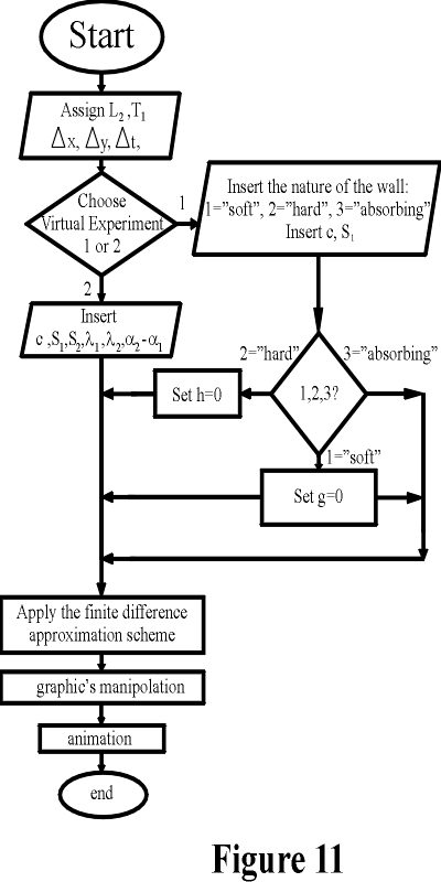
The finite differences scheme is roughly described as follows: let M, K be two positive integers and Dx = Dy = L₂/M, Dt = T₁/K be the discretization steps for the independent variables x, y, t respectively. We approximate the function value u(iDx, jDy, kDt) with the unknown u_i,j,k, i = 0,1,2,...,M, j = 0,1,2,...,M, k = 0,1,2,...,K. These unknowns u_i,j,k, i = 0,1,2,...,M, j = 0,1,2,...,M, k = 0,1,2,...,K are computed solving finite difference equations which are obtained approximating the mathematical model proposed. In particular the derivatives appearing in the model are approximated with finite differences, that is with incremental ratios. The finite differences approximation used is the simplest one and can be found in [3] p. 164-210. Note that in order to guarantee the validity of the finite differences approximation some conditions must be satisfied by Dx, Dy, Dt. In Figure 11 a flow chart of the "virtual laboratory" is shown.

4. Historic note and applications

This section is mainly devoted to the history of the study of reflection and interference phenomena in light propagation and in acoustics. The first study of reflection phenomena in light propagation can be retrieved to the ancient greeks in the treatise "Optics" of Euclid. In this treatise we can find a study of light propagation in straight lines, some elementary reflection laws, and a qualitative knowledge of reflection phenomena. That is Euclid introduced in his work some elementary notations and laws of geometrical optics. Only in the 17th century Christian Huygens (1629-1695) and Isaac Newton (1642-1726) produced a great effort in the study of diffraction and interference phenomena, that is two phenomena typical of physical (wave) optics. Huygens proposed the "wave" theory of light later called physical optics while Newton proposed the "particle" theory of light. During the 17th and 18th century Newton's theory prevaled over Huygens theory. The "particle" theory of light easily explained some interference phenomena (i.e.: for example Newton's rings). However the "particle" theory could not explain some interference phenomena and the diffraction of light. Finally in 1801 Thomas Young (1773-1829) performed an experiment that demonstrated the wave nature of light. This experiment made clear that Newton "particle" theory could explain reflection phenomena but not all interference phenomena, while Huygens "wave" theory could explain both reflection phenomena and interference phenomena. In 1801 Young's experiment proved that two overlapping light waves interfere with each other. Moreover in this experiment for the first time the wavelength of monochromatic light was measured (see Application 1) Young's experiment showed that the light passing through two closely spaced slits produce (Figure 12) a pattern of bright and dark fringes on a screen. The fringe pattern is a direct indication of the occurence of some interference phenomenon between the light waves coming from each slit.

These two narrow slits behave as two coherent sources of light waves. These waves interfere constructively and destructively at different points on the screen producing a pattern of alternating bright and dark regions. A different arrangement of Young's experiment is the following. A source generates monochromatic light. This monochromatic light passes successively through a spherical surface and an optically flat plate. The plate and the spherical surface are usually made of glass. The flat plate and the spherical surface are put in contact as shown in Figure 13.

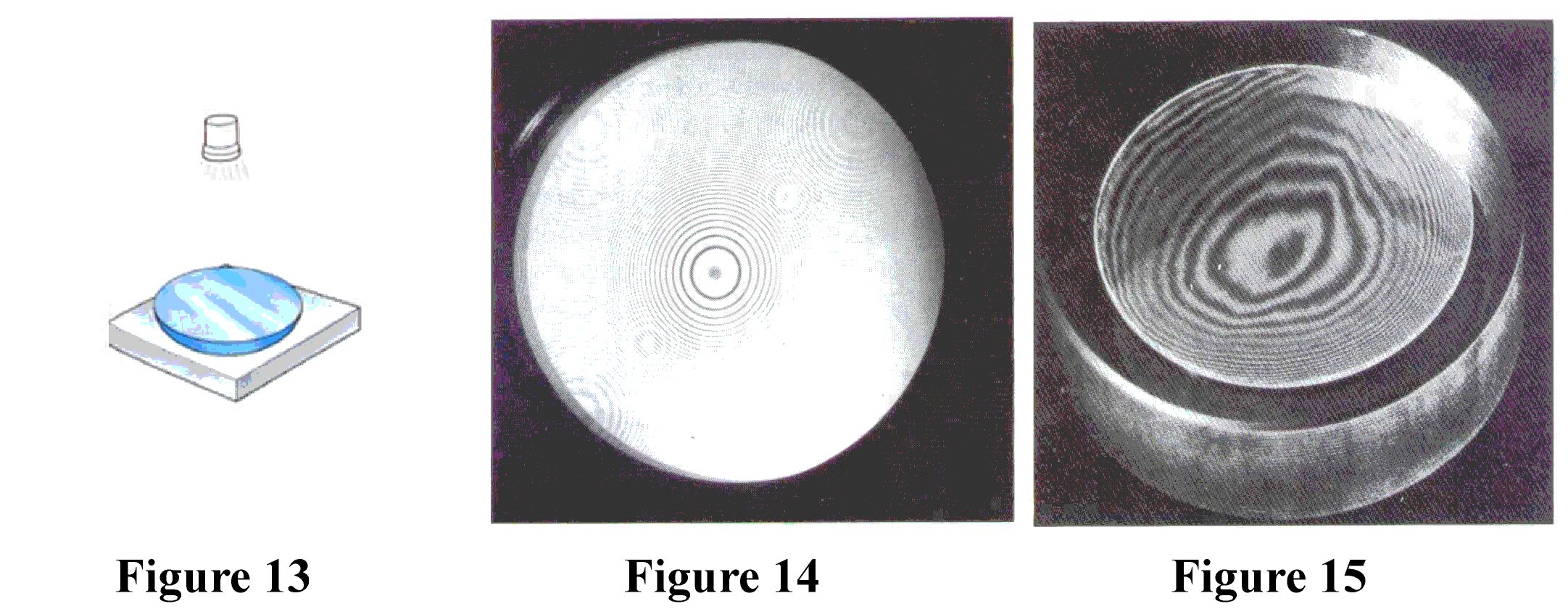
Due to interference phenomena we can see the well known Newton's rings (see Figure 14) on the spherical glass surface (see Figure 13), that is a pattern of circular interference rings. When the curved surface is irregular the interference fringes are not circular (see Figure 15). Analogously if the curved surface is substituted with a plane slightly inclined with respect to the flat plate, the wedge of air formed between the two plates causes an interference pattern consisting of straight fringes when the plate is flat and when the plate is not perfectly flat the pattern is wavy. We note that these experiments use a monochromatic light source, that is a source of time harmonic light. The natural light is not monochromatic, but monochromatic light can be produced in a laboratory and makes easier to observe these elementary interference phenomena.

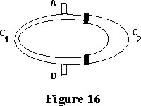
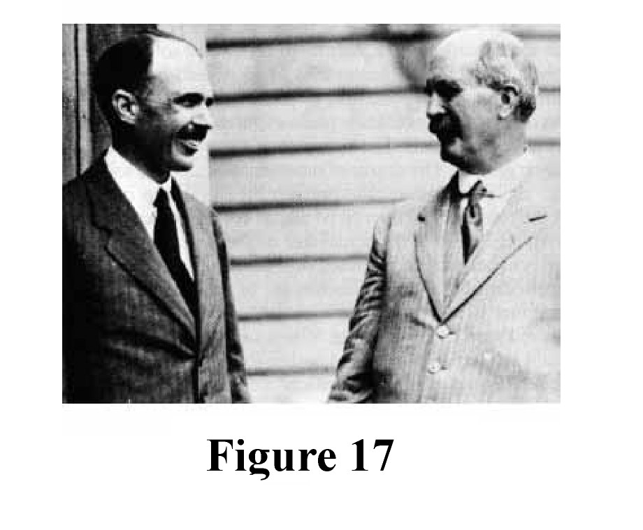
In the case of acoustic waves an experiment that shows an interference phenomenon can be carried out using Quincke's duct (see Figure 16) A diapason situated at the point A produces "monochromatic" acoustic waves propagating in the duct shown in Figure 16. These waves arrive at D, some of these trough the C₂-arc (see Figure 16), which is extensible, and some of them along the fixed C₁-arc. The experiment consists in arranging the extensible C₂-arc in such a way that there is no sound at the point D. When there is no sound at the point D then the distance covered by the waves to reach D going through C₁ and going through C₂ differs for a half integer number of wavelenghts. That is we have destructive interference at the point D. The optical and acoustic experiments described above provide a rough tool to measure the wavelenght of a monochromatic source of light or of sound. The wave theory of light propagation reached its full development with the work of James Clerk Maxwell (1831-1879). Maxwell used for the first time partial differential equations as the basic model of physics and developed work of Oliver Heaviside (1850-1925) in symbolic calculus to solve partial differential equations. In the 20th century William Henry Bragg (1862-1942) and his son William Laurence (1890-1971) (see Figure 17) studied the natural light spectrum, that is the spectrum of the sunlight. They used the interference of monochromatic waves to get the well known Bragg's law observing the so called Bragg's angles. Bragg's law was discovered in the study of chrystal structures. Moreover they studied high frequency spectrography. Bragg father and son got the Nobel prize in 1915 for their work.

We present three elementary applications of the interference phenomena studied above. The first application concerns the measurement of the wavelenght, the second one is a technique to test the flatness of a surface and finally the third one is a noise canceling technique used to reduce the disturbances in the transmission of signals.

Application 1: Wavelenght measurement. Given some bright fringes produced by a monochromatic wave passing through two slits situated at distance "a" one from the other (see Figure 12) on a screen located at distance L >> a from the slits. We have that the angle q for the interference maxima can be determined using Bragg's law (11): sin q = (n l)/2a, n = 0, ± 2, ± 4,... where the value of n specifies the order of the fringe. Observing the first order bright fringe (n=2) and knowing a we can estimate the wavelength l.

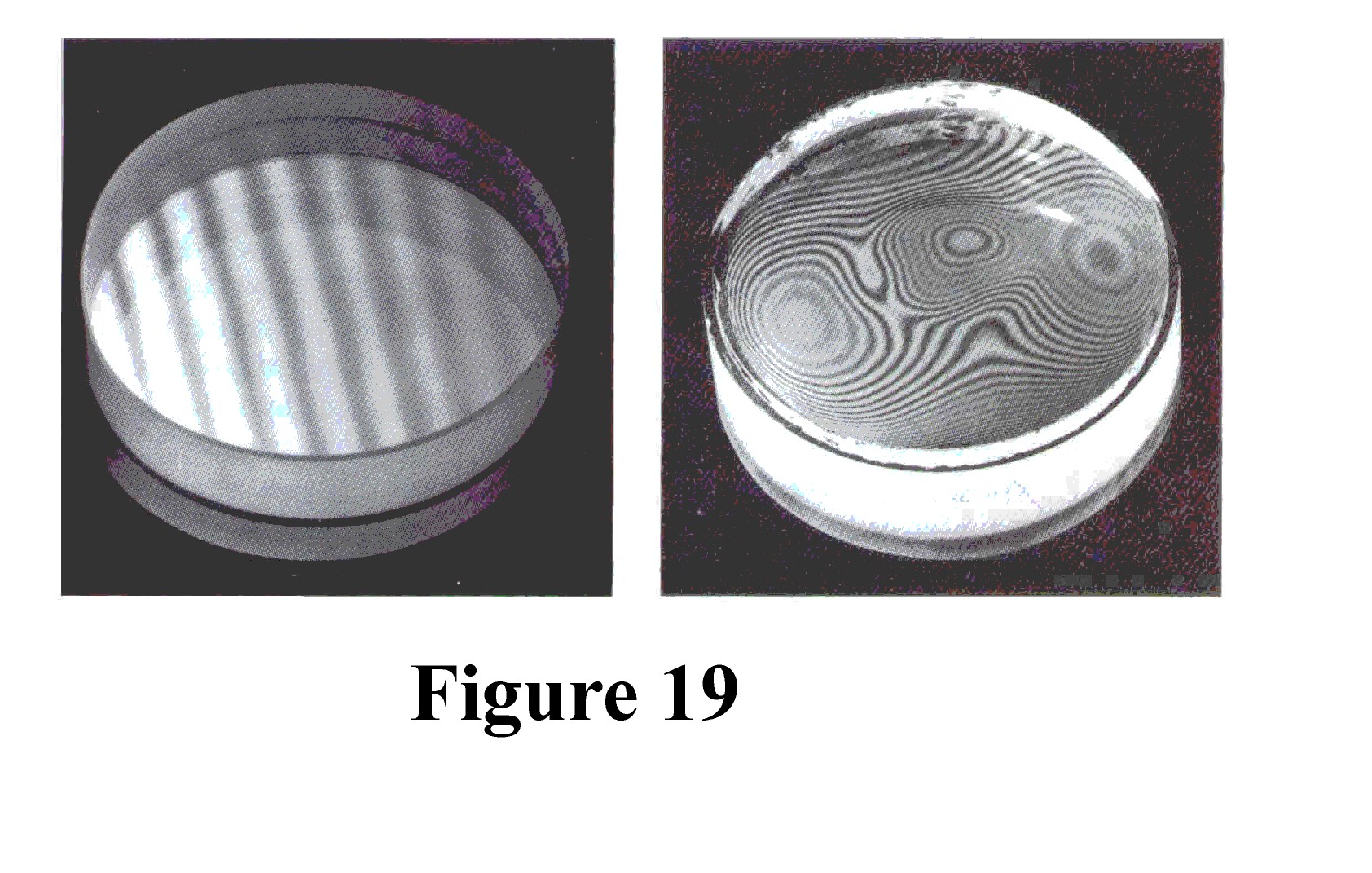
Application 2: Testing the flatness of a surface. Air wedge interference is used to test a surface for flatness. The surface to be tested S₁ is situated slightly inclined with respect to a flat plate S₂ in such a manner to leave an air wedge W between the two surfaces (see Figure 18). A light source (not necessarily monochromatic) falls on the suface S₁ and the wedge of air W causes reflected light to appear on the surface S₁ with an interference pattern of alternative dark and bright fringes. If the interference fringes observed are straight then the surface is flat otherwise the surface is not flat (see Figure 19). In another example an air wedge is used to establish the degree to which the surface of a lens or mirror is spherical. In fact when a spherical surface is put in contact with a flat plate and a light source is located over the spherical surface we can observe circular fringes of interference known as Newton's rings (see Figure 15).

Application 3: Noise canceling techniques. Destructive interference can be used for noise canceling for example in the headphones (see Figure 20). A microphone is mounted (see Figure 20) inside the headphones which contains a circuitry that processes the electronic signal coming from the microphone. When a noise is detected by the microphone then the circuitry reproduces the noise in a form that is exactly out of phase with the original noise. This "artificial" noise is played back through the headphones so that the destructive interference eliminates the disturbance.

References

[1] V.S.Vladimirov, " Equations of mathematical physics", 1971, Marcel Dekker Inc., New York.

[2] A.C.Reynolds, "Boundary conditions for the numerical solution of wave propagation problems", Geophysics 43, 1978, 1099-1110.

[3] A.R.Mitchell, D.F.Griffith, "The finite difference method in partial differential equations", 1980, John Wiley & Sons, New York.