The use of wavelets in the operator expansion method for time dependent acoustic obstacle scattering
Maria Cristina Recchioni
Istituto di Teoria delle Decisioni e Finanza Innovativa
Università di Ancona
Piazza Martelli 8, 60121 Ancona, Italy
e-mail : recchioni@posta.econ.unian.it
Francesco Zirilli
Dipartimento di Matematica "G. Castelnuovo"
Università di Roma "La Sapienza"
00185 Roma, Italy
e-mail : f.zirilli@caspur.it
In this paper we present a generalization of the "operator expansion method" developed in [1]. Let D contained R3 be a bounded simply connected domain with locally Lipschitz boundary. The boundary of D is characterized by a given boundary acoustic impedance not necessarily constant. The operator expansion method has been used to solve the exterior boundary value problem for the Helmholtz equation in R3\D via a "perturbative series". This perturbative series is built using two auxiliary "reference" surfaces. In [1] these surfaces are chosen to be the surfaces of two different spheres, the domain D to be starlike and the series expansion is built using the spherical coordinate system. The main advantage of these choices is that when the basis of the spherical harmonic functions is used to solve the problem the linear system involved in the computation of each term of the perturbative series is a diagonal linear system. However these choices do not guarantee the numerical convergence of the "perturbative series" when the shape of D is "far" from being the shape of a sphere. The new formulation proposed here involves more general reference surfaces, and a more general choice of the coordinate system used to build the expansion than the choice made previously of spherical coordinates. That is domains D, whose boundary is "far" from being the boundary of a sphere, are treated using as reference surfaces two surfaces "close" to the boundary of D. We show the numerical convergence of the associated "perturbative series". The price to be paid for this more general choice of reference surfaces is that a dense linear system must be solved to compute each term of the "perturbative series". To overcome this difficulty a suitable basis of wavelets [2] is used. The use of this basis reduces the solution of the dense linear systems mentioned above to the solution of very sparse linear systems. The numerical method obtained combining these ideas to solve the exterior boundary value problem for the Helmholtz equation is computationally highly parallelizable and is a practical tool to solve the time dependent problem when the wave equation with suitable conditions is considered. In fact the solution of the time dependent acoustic scattering problem can be computed as superposition of the solutions of several time harmonic acoustic scattering problems that is problems for the Helmholtz equation. We show some numerical experiments obtained using a parallel implementation of the computational method proposed. The speed up factor obtained as a function of the number of processors used is shown. Really impressive speed up factors are obtained. The data shown in Fig. 4.1d), that is the "submarine", have been taken from the website: http://avalon.viewpoint.com/. The data that define Obstacle 5 (Fig. 4.1e)) are a slight modification of the data of Fig. 4.1d). Obstacle 5 is one of the obstacles used to test the computational method proposed. We discuss the results obtained both from the quantitative and the qualitative point of view.
In the following gif animations we show from left to right the colour scale, the incident wave and the scattered wave.
In the following mpeg animations we show from left to right the incident wave and the scattered wave. These quantities are represented in the following colour scale:
Obstacles animations 1 (h=0.5) and 2 (h=2):
File mpeg - 876K )
File mpeg - 136K )
Obstacle animation 3:
File mpeg - 136K )
Obstacle animation 4:
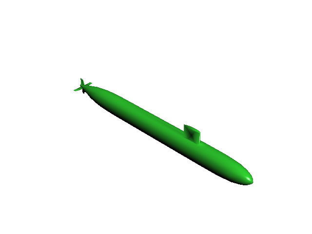
In the Animation 4 the obtacle is represented in the (x2,x3) plane. The x3 axis corresponds to the symmetry axis of the main body of the submarine, that is the direction of the maximum length of the obstacle.
File mpeg - 736K )