PAPER:
A numerical method to solve an acoustic inverse scattering problem involving ghost obstacles
Lorella Fatone
Dipartimento di Matematica Pura ed Applicata
Università di Modena e Reggio Emilia
Via Campi 213/b, 41100 Modena, Italy
Ph. N. +39-059-2055589, FAX N. +39-059-370513
e-mail : fatone.lorella@unimo.it
Maria Cristina Recchioni
Dipartimento di Scienze Sociali "D. Serrani"
Università Politecnica delle Marche
Piazza Martelli 8, 60121 Ancona, Italy
Ph. N. +39-071-2207066, FAX N. +39-071-2207150
e-mail : m.c.recchioni@univpm.it
Francesco Zirilli
Dipartimento di Matematica "G. Castelnuovo"
Università di Roma "La Sapienza"
Piazzale Aldo Moro 2, 00185 Roma, Italy
Ph. N. +39-06-49913282, FAX N. +39-06-44701007
e-mail : f.zirilli@caspur.it
- Abstract
- The inverse scattering problem
- A Numerical Experiment
- References
- Useful Links
1. Abstract
In [8] we study a time harmonic inverse acoustic scattering problem involving
an obstacle that when hit by an incoming acoustic wave tries to appear in a location in
space different from its actual location eventually with a shape and an acoustic boundary impedance different
from its actual ones. We refer to this problem as inverse ghost obstacle problem and to the scatterers of this type as
a special class of smart obstacles.
The term "ghost" comes from the fact that the smart obstacle, when hit by the incoming
wave, tries to appear as
a ghost obstacle, that is as a virtual obstacle in a location in space where no real obstacle is present.
We assume that the intersection between the obstacle and the ghost
obstacle is empty. The obstacle tries to produce this virtual image of itself
circulating on its boundary a suitable pressure current.
A pressure current is a quantity whose physical
dimension is pressure divided by time. The following time harmonic
inverse ghost obstacle scattering problem is considered: from the
knowledge
of several far fields generated by the smart obstacle when hit by
known time harmonic waves, of its acoustic boundary impedance and of the acoustic boundary impedance of the
ghost obstacle find the location of the
smart obstacle, that is find a point in the interior of the smart
obstacle and eventually find the shape of the smart obstacle.
The method proposed to solve this problem is a generalization of the
well known Herglotz function method. We present some numerical experiments based on synthetic data that are used to test
the numerical method
introduced here.
This website contains some auxiliary material that helps the understanding
of the paper [8].
2. The inverse scattering problem
We consider a time harmonic acoustic inverse
scattering problem involving a smart obstacle that when hit by an
incoming wave pursues the goal of appearing in a location in
space different from its actual location eventually with a shape
and an acoustic boundary impedance different from its actual ones.
The obstacle pursues this goal circulating a pressure current on
its boundary. A pressure current is a quantity whose physical
dimension is pressure divided by time. This type of obstacles is
a special class of smart obstacles. Mathematical models of time
dependent and time harmonic acoustic and electromagnetic direct
scattering problems involving smart obstacles have been proposed
in [1]-[8]. In the time
dependent acoustic case these models are optimal
control problems for the wave equation where the pressure current
mentioned above plays the role of the control variable. In the
time harmonic acoustic case these models reduce to a constrained
optimization problem with the constraints given by an exterior
boundary value problem for the Helmholtz equation with the space dependent
part of a time harmonic pressure current as independent variable
of the optimization problem. The solution of the optimal control
problem is obtained formulating the first order necessary optimality condition via the
Pontryagin maximum principle while the solution of the
constrained optimization problem is obtained formulating the
first order necessary optimality condition using the Lagrangian
functional. The first order optimality conditions obtained are
solved numerically.
We consider the following inverse problem:
Time Harmonic Ghost Obstacle Inverse Scattering
Problem:
From the knowledge of several far fields
generated by the smart obstacle when hit by known incident
acoustic waves, the knowledge of the boundary acoustic impedances
of the smart obstacle and of the ghost obstacle
find the
location of the smart obstacle, that is find a point in the
interior of the smart obstacle and, eventually find its shape.
Note that we assume that the intersection between the smart
obstacle and the ghost obstacle is empty. Obviously the solution
of an inverse problem involving a smart obstacle is more difficult
than the solution of the analogous problem involving a passive
obstacle, that is an obstacle that does not react pursuing an
assigned goal when hit by an incoming wave. The degree of
difficulty of the inverse problem for the smart obstacle increases
with the ability of the obstacle of pursuing its goal.
The classical inverse problem for a passive obstacle can be
formulated as follows:
Acoustic Time Harmonic (Passive) Inverse Scattering Problem: From the knowledge of
the far fields generated by the (passive) obstacle when hit by several known
incoming time harmonic waves and of the acoustic boundary impedance of the obstacle, determine the boundary of the
obstacle.
This last problem and several related problems have been widely
investigated and many efficient computational methods have been
developed for their solution (see for example [9], [10],
[11] and the references therein) while the
formulation of mathematical models for inverse scattering problems
involving smart obstacles and the development of numerical methods
to solve them are rather unexplored research fields. Recently the
authors and a co-author have formulated mathematical models for
inverse problems and developed numerical methods to solve inverse
scattering problems when smart obstacles that pursue the goal of
being undetectable (i.e.:furtive obstacles) or of appearing with a
shape and/or boundary impedance different from their actual ones
(i.e.: masked obstacles) are considered (see [4],
[7]). An inverse scattering problem involving an
obstacle that tries to appear in a location different from its
actual one (i.e.: ghost obstacle) has been proposed in
[5] where the solution of the inverse problem has
been obtained with an iterative procedure that minimizes a
suitable functional. The evaluation of this functional implies the
solution of a direct scattering problem for the smart obstacle.
Here we develop a new approach to solve this last inverse
problem in particular we develop an ad hoc Herglotz wave function
method that generalizes the Herglotz wave function method
introduced in [7] to solve inverse problems involving
furtive or masked obstacles.
The method proposed to solve the
inverse ghost problem is an iterative procedure that does not
require the solution of a direct scattering problem at each
iteration and that it is based on the minimization of a suitable
functional defined via the vector Herglotz wave function.
The method proposed here
when compared to the numerical method proposed in
[7] has the advantage of being computationally much more efficient. The main
difficulty that we must overcome in developing this method
consists in the fact that the far field measures are taken in a
coordinate system with origin in a point that we choose in the
interior of the ghost obstacle and not with origin in a point in the
interior of the smart obstacle. Hence the new formulation of the
Herglotz wave function method must take into account this fact and
it must consider as unknowns the coordinates of a point in the
interior of the ghost obstacle (i.e. for example the center of mass of the
boundary of the ghost obstacle) in a coordinate system having the origin in
a point in the interior of the smart obstacle (i.e. for example
the center of mass of the boundary of the smart obstacle). We
assume that the obstacle and the ghost obstacle are such that they contain
the centers of mass of their boundaries.
The choice of taking the center of mass of the boundary of the obstacle
as origin is made only for simplicity and any other point in the
interior of the obstacle can be used without substantial changes.
We note that we assume that the smart obstacle is a starlike set
with respect to the center of mass of its boundary. This
assumption is due to the particular mathematical formulation of
the direct ghost obstacle scattering problem used and can be
substituted with other assumptions.
3. A Numerical Experiment
Let (r, q, n)
be the canonical spherical coordinate system with pole in the orgin of the Cartesian coordinate system
shown in Figure 1.
The setting of the numerical experiment consists in an acoustically soft (i.e. c=0) smart
sphere
of radius one (i.e. the smart obstacle W) (see Figure 1) that tries to
appear outside a shere of radius 2.4 that will be called Wa*
(see Figure 1) as an acoustically soft
(i..e. cG=0) sphere of radius 0.5 (i.e. the ghost obstacle WG) in a location
in space different from its actual one (see Figure 1). The smart sphere is hit by an incoming plane wave
of the form:
where k=1, c=1,
a=(sinqcosn,
sinqsinn,cosq)T where
0 ≤ q ≤ p,
0 ≤ n < 2p, for some choices of the incoming direction
a.
In particular the ghost sphere has center in the
point of cartesian coordinates (1.7,0,0)T in the frame that has
the origin the center of mass of the smart obstacle.
The boundary of the sphere of radius 2.4 will be denoted in the following with
We, e =1.4.
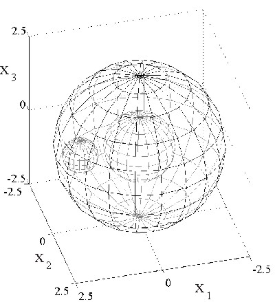 |
Figure 1: The
numerical experiment: W=sphere of radius one,
WG=sphere of radius 0.5,
W*a=We=sphere of radius 2.4.
|
Let qi = ip/10, i = 1,2,¼,9, fj = 2jp/10,
j = 1,2,¼,9 and let us denote with
xe(q,f) a
point of ¶We. Table 1 shows how the field
scattered by the smart obstacle resembles the one scattered by the
ghost obstacle. That is shows how much the smart obstacle has achieved its
goal. We compute the fields
usk,
a(
xe(qi,fj)),
usG,k,
a(
xe(qi,fj)),
usp,k,
a(
xe(qi,fj)),
xe(qi,fj) = (1+e)(sinqicosfj,sinqisinfj,cosqi)T
Î ¶We,
e = 1.4, i = 1,2,¼, 9, j = 1,2,¼,9 scattered by the
smart obstacle, by the ghost obstacle and by the passive obstacle
respectively when hit by a harmonic plane wave (1) with c = 1, k = 1,
a = (sinq*cosf*,sinq*sinf*,cosq*)T
for several choices of q*, f* as shown in Table
1. We consider the following quantities:
|
Esmart(q*,f* |
) = |
æ
ç
ç
ç
ç
ç
è
|
|
|
|
9
å
i = 1
|
|
9
å
j = 1
|
|usk,
a(
xe(qi,fj))-usG,k,
a(
xe(qi,fj))|2 |
|
|
9
å
i = 1
|
|
9
å
j = 1
|
|usG,k,
a(
xe(qi,fj))|2 |
|
|
ö
÷
÷
÷
÷
÷
ø
|
1/2
|
, |
| (2) |
|
Epassive(q*,f* |
) = |
æ
ç
ç
ç
ç
ç
è
|
|
|
|
9
å
i = 1
|
|
9
å
j = 1
|
|usp,k,
a(
xe(qi,fj))-usG,k,
a(
xe(qi,fj))|2 |
|
|
9
å
i = 1
|
|
9
å
j = 1
|
|usG,k,
a(
xe(qi,fj))|2 |
|
|
ö
÷
÷
÷
÷
÷
ø
|
1/2
|
. |
| (3) |
Note that the quantities (2) and (3) are
measures of how the field usk,
a and
usp,k,
a resemble to the field scattered by the ghost
obstacle.
The parameters l,
V that appear in Table 1 are parameters that appear in the
objective function (assigned goal) of the smart obstacle (see [8] for further details).
|
| l = 0.5, V = 1
|
|
|
|
q* | f* | ESmart | EPassive
|
|
p/5 |
p/4 | 0.630 | 1.861
|
|
2p/5 | p/4 | 0.582 | 1.871
|
|
p/2 | p/2 | 0.593 | 1.801 |
| l = 0.8, V = 1
|
|
|
|
q* | f* | ESmart | EPassive
|
|
p/5 |
p/4 | 0.332 | 1.861
|
|
2p/5 | p/4 | 0.341 | 1.871
|
|
p/2 | p/2 | 0.321 | 1.801 |
Table 1: Comparison between the acoustic fields scattered by the
ghost obstacle and by the smart obstacle (ESmart) and
comparison between the acoustic fields scattered by the ghost
obstacle and by the passive obstacle (EPassive)
Table 1 shows that the quantity Esmart is smaller than the
quantity Epassive and the quantity Esmart decreases when
l increases, that is shows that the smart obstacle is
achieving its goal.
As discussed in [8] the parameter l
is such that 0≤ l ≤ 1
and when l increases the ability of the smart obstacle of pursuing its goal increases.
The following virtual reality animation shows the approximation of the point in the interior of
the smart obstacle generated by the iterative procedure described in [8].
The setting of the experiment is shown in Figure 1. We work in a spherical coordinate system
with pole in a point G in the interior of the ghost obstacle. This assumption is made for simplicity and we take G to be
the center of mass of the ghost obstacle (i.e. the sphere of radius 0.5). The aim of the inverse procedure is to determine
a point in the interior of the smart obstacle, in particular we want to determine the center of mass S of the boundary of
the smart obstacle. Hence the unknown that we want to determine consists in the vector p that joins the point G
to the point S. The solution of the inverse problem is the vector p=(-1.7,0,0)T.
The initial guess p* for the location of
the center of mass of the smart obstacle is chosen to be the center of mass of the boundary
of the ghost obstacle that is p*=0.
The initial guess of the boundary of the smart
obstacle has been chosen to be a sphere of radius 2 having its center in the approximation of the
point S given by G+p*.=G
Moreover we choose
c = 1, l = 0.9, m = 1-l, V = 1 (see [8] ).
The far field measurements are affected by a noise of 1% that is
we consider the measures
F0,u,
p(
x,k,
a)(1+Er(
x,k,
a)),
x=(sinqcosn,
sinqsinn,cosq)T where
0 ≤ q ≤ p,
0 ≤ n < 2p,
where Er is a random variable uniformly distributed in [-10-2,10-2],
and F0,u,
p(x,k,
a) is computed solving
numerically the direct problem.
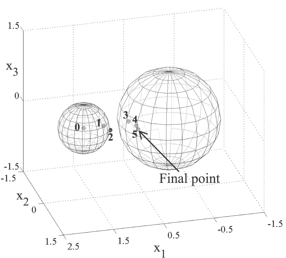
Table 2 shows from left to right the number of iteration
i, the cartesian components p1*, p2*, p3* of
the current approximation
p* of the vector p. The sequence of the p* computed in the iteration
is shown in Figure 2. . Note that from the seventh iteration (i.e. the point numbered with 3 in Figure 2) the point
G+p* is in the interior of the smart obstacle.
|
iteration i | p1* | p2* | p3*
|
|
0 | 0 | 0 | 0 |
|
5 | -0.776 | -0.0007 | -0.0008
|
|
6 | -0.776 | -0.203 | -0.203 |
|
9 | -1.089 | -0.146 | -0.148 |
|
12 | -1.204 | -0.443 | -0.372
|
Table 2: Approximations p* of p
Figure 2: Sequence
of points generated by the inversion algorithm. The initial point
used by the algorithm is the center of the sphere of radius 0.05 numbered with 0
that is the center of mass of the ghost obstacle.
Some of the points generated by the algorithm are shown as spheres
of radius 0.05. These points are numbered progressively to show
the order in which they are generated by the algorithm.
Finally we present a virtual reality animation of the numerical experiment discussed above to help the understanding
of the behaviour of the reconstruction procedure.
The virtual reality animation consists in four windows. Three windows are static windows showing the ghost obstacle,
the smart obstacle and the setting of the experiment.
The remaining window is a dynamic window showing how the reconstruction of the point in the interior of the smart obstacle
takes place.
Video clip: animated reconstruction ghost obstacle inverse scattering problem
click here to download
4. References
- [1]
-
L. Fatone, M. C. Recchioni and F. Zirilli,
"A masking
problem in time dependent acoustic obstacle scattering",
ARLO - Acoustics Research Letters Online, 5, Issue 2, 25-30 (2004).
- [2]
- L. Fatone, M. C. Recchioni and F. Zirilli, "Furtivity
and masking problems in time dependent electromagnetic obstacle
scattering", Journal of Optimization Theory and Applications, 121,
223-257 (2004).
- [3]
- F. Mariani, M. C. Recchioni and F. Zirilli,"The use of the Pontryagin
maximum principle in a furtivity problem in time-dependent
acoustic obstacle scattering", Waves in Random Media,
11, 549-575 (2001).
- [4]
- L. Fatone, M. C. Recchioni, A. Scoccia and F. Zirilli, "Direct and inverse scattering
problems involving smart obstacles", Journal of Inverse and Ill Posed Problems, 13, 247-257 (2005).
- [5]
-
L. Fatone, M. C. Recchioni and F. Zirilli, "New scattering problems and numerical methods in acoustics"
in Recent Research Developments in Acoustics, S.G. Pandalai Managing Editor, Transworld Research Network,
Kerala India, Vol. II, 2005, 39-69.
- [6]
- L. Fatone, G. Pacelli,
M. C. Recchioni and F. Zirilli, "The use of optimal control methods to
study two new classes of smart obstacles in time dependent acoustic scattering",
to appear in Journal of Engineering Mathematics (2006).
- [7]
-
L. Fatone, M. C. Recchioni and F. Zirilli, "A method to solve an acoustic inverse scattering problem involving smart
obstacles", to appear in Waves in Random and Complex Media (2006).
- [8]
-
L. Fatone, M. C. Recchioni and F. Zirilli, "A numerical method to solve an acoustic inverse scattering problem
involving ghost obstacles",
submitted to
Journal of Inverse and Ill Posed Problems (2006).
- [9]
- D. Colton, J. Coyle and P. Monk, "Recent developments in inverse acoustic scattering", SIAM
Review, 42, 369-414 (2000).
- [10]
- D. Colton and R. Kress, Inverse Acoustic and Electromagnetic Scattering
Theory, Springer Verlag, Berlin, 1992.
- [11]
- L. Misici and F. Zirilli, "Three-dimensional inverse
obstacle scattering for time harmonic waves: a numerical method",
SIAM Journal on Scientific Computing, 15, 1174-1189 (1994).
5. Useful Links
http://www.econ.univpm.it/recchioni/
http://www.econ.univpm.it/recchioni/w6
http://www.econ.univpm.it/recchioni/w9
http://www.econ.univpm.it/recchioni/w10
http://www.econ.univpm.it/recchioni/w11
http://www.econ.univpm.it/recchioni/w12
http://www.econ.univpm.it/recchioni/w13
Entry n.